Quantopian Overview
Quantopian provides you with everything you need to write a high-quality algorithmic trading strategy. Here, you can do your research using a variety of data sources, test your strategy over historical data, and then test it going forward with live data. Top-performing algorithms will be offered investment allocations, and those algorithm authors will share in the profits.
Important Concepts
The Quantopian platform consists of several linked components. The Quantopian Research platform is an IPython notebook environment that is used for research and data analysis during algorithm creation. It is also used for analyzing the past performance of algorithms. The IDE (interactive development environment) is used for writing algorithms and kicking off backtests using historical data. Algorithms can also be simulated using live data, also known as paper trading. All of these tools use the data provided by Quantopian: US equity price and volumes (minute frequency), US futures price and volumes (minute frequency), US equity corporate fundamentals, and dozens of other integrated data sources.
This section covers each of these components and concepts in greater detail.
Data Sources
We have minute-bar historical data for US equities and US futures since 2002 up to the most recently completed trading day (data uploaded nightly).
A minute bar is a summary of an asset's trading activity for a one-minute period, and gives you the opening price, closing price, high price, low price, and trading volume during that minute. All of our datasets are point-in-time, which is important for backtest accuracy. Since our event-based system sends trading events to you serially, your algorithm receives accurate historical data without any bias towards the present.
During algorithm simulation, Quantopian uses as-traded prices. That means that when your algorithm asks for a price of a specific asset, it gets the price of that asset at the time of the simulation. For futures, as-traded prices are derived from electronic trade data.
When your algorithm calls for historical equity price or volume data, it is adjusted for splits, mergers, and dividends as of the current simulation date. In other words, if your algorithm asks for a historical window of prices, and there is a split in the middle of that window, the first part of that window will be adjusted for the split. This adjustment is done so that your algorithm can do meaningful calculations using the values in the window.
Quantopian also provides access to fundamental data, free of charge. The data, from Morningstar, consists of over 600 metrics measuring the financial performance of companies and is derived from their public filings. The most common use of this data is to filter down to a sub-set of securities for use in an algorithm. It is common to use the fundamentals metrics within the trading logic of the algorithm.
In addition to pricing and fundamental data, we offer a host of partner datasets. Combining signals found in a wide variety of datasets is a powerful way to create a high-quality algorithm. The datasets available include market-wide indicators like sentiment analysis, as well as industry-specific indicators like clinical trial data.
Each dataset has a limited set of data available for free; full datasets available for purchase, a la carte, for a monthly fee. The complete list of datasets is available here.
Our US equities database includes all stocks and ETFs that traded since 2002, even ones that are no longer traded. This is very important because it helps you avoid survivorship bias in your algorithm. Databases that omit securities that are no longer traded ignore bankruptcies and other important events, and lead to false optimism about an algorithm. For example, LEH (Lehman Brothers) is a security in which your algorithm can trade in 2008, even though the company no longer exists today; Lehman's bankruptcy was a major event that affected many algorithms at the time.
Self-Serve Data allows you to upload your own time-series csv data to Quantopian. In order to accurately represent your data in pipeline and avoid lookahead bias, your data will be collected, stored, and surfaced in a point-in-time nature similar to Quantopian Partner Data.
Our US futures database includes 72 futures. The list includes commodity, interest rate, equity, and currency futures. 24 hour data is available for these futures, 5 days a week (Sunday at 6pm - Friday at 6pm ET). Some of these futures have stopped trading since 2002, but are available in research and algorithms to help you avoid survivorship bias.
There are many other financial data sources we'd like to incorporate, such as options and non-US markets. What kind of data sources would you like us to have? Let us know.
Research Environment
The research environment is a customized IPython server. With this open-ended platform, you are free to explore new investing ideas. For most people, the hardest part of writing a good algorithm is finding the idea or pricing "edge." The research environment is the place to do that kind of research and analysis. In the research environment you have access to all of Quantopian's data- price, volume, corporate fundamentals, and partner datasets including sentiment data, earnings calendars, and more.
The research environment is also useful for analyzing the performance of backtests and live trading algorithms. You can load the result of a backtest or live algorithm into research, analyze results, and compare to other algorithms' performances.
IDE and Backtesting
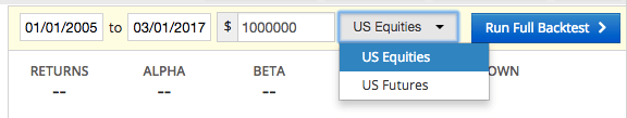
The IDE (interactive development environment) is where you write your algorithm. It's also where you kick off backtests. Pressing "Build" will check your code for syntax errors and run a backtest right there in the IDE. Pressing "Full Backtest" runs a backtest that is saved and accessible for future analysis.
The IDE is covered in more detail later in this help document.
Paper Trading
Paper trading is also sometimes known as walk-forward, or out-of-sample testing. In paper trading, your algorithm gets live market data (actually, 15-minute delayed data) and 'trades' against the live data with a simulated portfolio. This is a good test for any algorithm. If you inadvertently overfit during your algorithm development process, paper trading will often reveal the problem. You can simulate trades for free, with no risks, against the current market on Quantopian.
Quantopian paper trading uses the same order-fulfillment logic as a regular backtest, including the slippage model.
Before you can paper trade your algorithm, you must run a full backtest. Go to your algorithm and click the 'Full Backtest' button. Once that backtest is complete, you will see a 'Live Trade’ button. When you start paper trading, you will be prompted to specify the amount of money used in the strategy. Note that this cash amount is not enforced - it is used solely to calculate your algorithm's returns.
Paper trading is currently only available for US equity trading.
Privacy and Security
We take privacy and security extremely seriously. All trading algorithms and backtest results you generate inside Quantopian are owned by you. You can, of course, choose to share your intellectual property with the community, or choose to grant Quantopian permission to see your code for troubleshooting. We will not access your algorithm without your permission except for unusual cases, such as protecting the platform's security.
Our platform is run on a cloud infrastructure.
Specifically, our security layers include:
- Never storing your password in plaintext in our database
- SSL encryption for the Quantopian application
- Secure websocket communication for the backtest data
- Encrypting all trading algorithms and other proprietary information before writing them to our database
We want to be very transparent about our security measures. Don't hesitate to email us with any questions or concerns.
Two-Factor Authentication
Two-factor authentication (2FA) is a security mechanism to protect your account. When 2FA is enabled, your account requires both a password and an authentication code you generate on your smart phone.
With 2FA enabled, the only way someone can sign into your account is if they know both your password and have access to your phone (or backup codes). We strongly urge you to turn on 2FA to protect the safety of your account.
How does it work?
Once you enable 2FA, you will still enter your password as you normally do when logging into Quantopian. Then you will be asked to enter an authentication code. This code can be either generated by the Google Authenticator app on your smartphone, or sent as a text message (SMS).
If you lose your phone, you will need to use a backup code to log into your account. It's very important that you get your backup code as soon as you enable 2FA. If you don't have your phone, and you don't have your backup code, you won't be able to log in. Make sure to save your backup code in a safe place!
You can setup 2FA via SMS or Google Authenticator, or both. These methods require a smartphone and you can switch between them at any time. To use the SMS option you need a US-based phone number, beginning with the country code +1.
To configure 2FA via SMS:
- Go to Account Settings and click 'Configure via SMS'.
- Enter your phone number. Note: Only US-based phone numbers are allowed for the SMS option. Standard messaging rates apply.
- You'll receive a 5 or 6 digit security token on your mobile. Enter this code in the pop-on screen to verify your device. Once verified, you'll need to provide the security token sent via SMS every time you login to Quantopian.
- Download your backup login code in case you lose your mobile device. Without your phone and backup code, you will not be able to access your Quantopian account.
To configure 2FA via Google Authenticator:
- Go to Two-Factor Auth and click 'Configure Google Authenticator'.
- If you don’t have Google Authenticator, go to your App Store and download the free app. Once installed, open the app, click 'Add an Account', then 'Scan a barcode'.
- Hold the app up to your computer screen and scan the QR code. Enter the Quantopian security token from the Google Authenticator app.
- Copy your backup login code in case you lose your mobile device. Without your phone and backup code, you will not be able to access your Quantopian account.
Backup login code
If you lose your phone and can’t login via SMS or Google Authenticator, your last resort is to login using your backup login code. Without your phone and this code, you will not be able to login to your Quantopian account.
To save your backup code:
- Go to https://www.quantopian.com/account?page=twofactor
- Click 'View backup login code'.
- Enter your security token received via SMS or on your Google Authenticator app.
- Copy your backup code to a safe location.
Developing in the IDE
Quantopian's Python IDE is where you develop your trading ideas. The standard features (tab completion, autosave, fullscreen, font size, color theme) help make your experience as smooth as possible.
Your work is automatically saved every 10 seconds, and you can click Save to manually save at any time. We'll also warn you if you navigate away from the IDE page while there's unsaved content. Tab completion is also available in the IDE, and can be enabled from the settings button on the top right.
Overview
We have a simple but powerful API for you to use:
initialize(context) is a required setup method for initializing state or other bookkeeping. This method is called only once at the beginning of your algorithm. context is an augmented Python dictionary used for maintaining state during your backtest or live trading session. context should be used instead of global variables in the algorithm. Properties can be accessed using dot notation (context.some_property).
handle_data(context, data) is an optional method that is called every minute. Your algorithm uses data to get individual prices and windows of prices for one or more assets. handle_data(context, data) should be rarely used; most algorithm functions should be run in scheduled functions.
before_trading_start(context, data) is an optional method called once a day, before the market opens. Your algorithm can select securities to trade using Pipeline, or do other once-per-day calculations.
Your algorithm can have other Python methods. For example, you might have a scheduled function call a utility method to do some calculations.
For more information, jump to the API Documentation section below. These core functions are also covered in Core Functions in the Getting Started Tutorial.
Manual Asset Lookup
Equities
If you want to manually select an equity, you can use the symbol function to look up a security by its ticker or company name. Using the symbol method brings up a search box that shows you the top results for your query.

To reference multiple securities in your algorithm, call the symbols function to create a list of securities. Note the pluralization! The function can accept a list of up to 500 securities and its parameters are not case sensitive.
Sometimes, tickers are reused over time as companies delist and new ones begin trading. For example, G used to refer to Gillette but now refers to Genpact. If a ticker was reused by multiple companies, use set_symbol_lookup_date('YYYY-MM-DD') to specify what date to use when resolving conflicts. This date needs to be set before any calls to symbol or symbols.

Another option to manually enter securities is to use the sid function. All securities have a unique security id (SID) in our system. Since symbols may be reused among exchanges, this prevents any confusion and verifies you are calling the desired security. You can use our sid method to look up a security by its id, symbol, or name.

In other words, sid(24) is equivalent to symbol('AAPL') or Apple.
Quantopian's backtester makes a best effort to automatically adjust the backtest's start or end dates to accommodate the assets that are being used. For example, if you're trying to run a backtest with Tesla in 2004, the backtest will suggest you begin on June 28, 2010 the first day the security traded. This ability is significantly decreased when using symbol instead of sid.
The symbol and symbols methods accept only string literals as parameters. The sid method accepts only an integer literal as a parameter. A static analysis is run on the code to quickly retrieve data needed for the backtest.
Manually looking up equities is covered in Referencing Securities in the Getting Started Tutorial.
Futures
To manually select a future in your algorithm, you probably want to reference the corresponding continuous future. Continuous futures are objects that stitch together consecutive contracts of a particular underlying asset. The continuous_future function can be used to reference a continuous future. The continuous_future function has auto-complete similar to symbol

Continuous futures maintain a reference to the active contract of an underlying asset, but cannot themselves be traded. To trade a particular future contract, you can get the current contract of a continuous future. This is covered in the Futures Tutorial.
Futures contracts can be looked up manually with future_symbol by passing a string for the particular contract (e.g. future_symbol('CLF16'). This is uncommon outside of research given the short lifetime of contracts.
Trading Calendars
Before running an algorithm, you will need to select which calendar you want to trade on. Currently, there are two calendars: the US Equities Calendar and the US Futures Calendar.
The US Equity calendar runs weekdays from 9:30AM-4PM Eastern Time and respects the US stock market holiday schedule, including partial days. Futures trading is not supported on the US Equity calendar.
The US Futures calendar runs weekdays from 6:30AM-5PM Eastern Time and respects the futures exchange holidays observed by all US futures (US New Years Day, Good Friday, Christmas). Trading futures and equities are both supported on the US Futures calendar.
To choose a calendar, select it from the dropdown in the IDE before running a backtest.
Scheduling Functions
Your algorithm will run much faster if it doesn't have to do work every single minute. We provide the schedule_function method that lets your algorithm specify when methods are run by using date and/or time rules. All scheduling must be done from within the initialize method.
def initialize(context):
  schedule_function(
    func=myfunc,
    date_rule=date_rules.every_day(),
    time_rule=time_rules.market_close(minutes=1),
    half_days=True
  )
For a condensed introduction to scheduling functions, check out the Scheduling Functions lesson in the Getting Started Tutorial.
Monthly modes (month_start and month_end) accept a days_offset parameter to offset the function execution by a specific number of trading days from the beginning and end of the month, respectively. In monthly mode, all day calculations are done using trading days for your selected trading calendar. If the offset exceeds the number of trading days in a month, the function isn't run during that month.
Weekly modes (week_start and week_end) also accept a days_offset parameter. If the function execution is scheduled for a market holiday and there is at least one more trading day in the week, the function will run on the next trading day. If there are no more trading days in the week, the function is not run during that week.
Specific times for relative rules such as 'market open' or 'market close' will depend on the calendar that is selected before running a backtest. If you would like to schedule a function according to the time rules of a different calendar, you can specify a calendar argument. To specify a calendar, you must import calendars from the quantopian.algorithm module.
If calendars.US_EQUITIES is used, market open is usually 9:30AM ET and market close is usually 4PM ET.
If calendars.US_FUTURES is used, market open is at 6:30AM ET and market close is at 5PM ET.
from quantopian.algorithm import calendars

def initialize(context):
  schedule_function(
    func=myfunc,
    date_rule=date_rules.every_day(),
    time_rule=time_rules.market_close(minutes=1),
    calendar=calendars.US_EQUITIES
  )
To schedule a function more frequently, you can use multiple schedule_function calls. For instance, you can schedule a function to run every 30 minutes, every three days, or at the beginning of the day and the middle of the day.
Scheduled functions are not asynchronous. If two scheduled functions are supposed to run at the same time, they will happen sequentially, in the order in which they were created.
Note: The handle_data function runs before any functions scheduled to run in the same minute. Also, scheduled functions have the same timeout restrictions as handle_data, i.e., the total amount of time taken up by handle_data and any scheduled functions for the same minute can't exceed 50 seconds.
Below are the options for date rules and time rules for a function. For more details, go to the API overview.


Date Rules
Every Day
Runs the function once per trading day. The example below calls myfunc every morning, 15 minutes after the market opens. The exact time will depend on the calendar you are using. For the US Equity calendar, the first minute runs from 9:30-9:31AM Eastern Time. On the US Futures calendar, the first minute usually runs from 6:30-6:31AM ET.
def initialize(context):
  # Algorithm will call myfunc every day 15 minutes after the market opens
  schedule_function(
    myfunc,
    date_rules.every_day(),
    time_rules.market_open(minutes=15)
  )

def myfunc(context,data):
  pass
Week Start
Runs the function once per calendar week. By default, the function runs on the first trading day of the week. You can add an optional offset from the start of the week to choose another day. The example below calls myfunc once per week, on the second day of the week, 3 hours and 10 minutes after the market opens.
def initialize(context):
  # Algorithm will call myfunc once per week, on the second day of the week,
  # 3 hours and 10 minutes after the market opens
  schedule_function(
    myfunc,
    date_rules.week_start(days_offset=1),
    time_rules.market_open(hours=3, minutes=10)
  )

def myfunc(context,data):
  pass
Week End
Runs the function once per calendar week. By default, the function runs on the last trading day of the week. You can add an optional offset, from the end of the week, to choose the trading day of the week. The example below calls myfunc once per week, on the second-to-last day of the week, 1 hour after the market opens.
def initialize(context):
  # Algorithm will call myfunc once per week, on the last day of the week,
  # 1 hour after the market opens
  schedule_function(
    myfunc,
    date_rules.week_end(days_offset=1),
    time_rules.market_open(hours=1)
  )

def myfunc(context,data):
  pass
Month Start
Runs the function once per calendar month. By default, the function runs on the first trading day of each month. You can add an optional offset from the start of the month, counted in trading days (not calendar days).
The example below calls myfunc once per month, on the second trading day of the month, 30 minutes after the market opens.
def initialize(context):
  # Algorithm will call myfunc once per month, on the second day of the month,
  # 30 minutes after the market opens
  schedule_function(
    myfunc,
    date_rules.month_start(days_offset=1),
    time_rules.market_open(minutes=30)
  )

def myfunc(context,data):
  pass
Month End
Runs the function once per calendar month. By default, the function runs on the last trading day of each month. You can add an optional offset from the end of the month, counted in trading days. The example below calls myfunc once per month, on the third-to-last trading day of the month, 15 minutes after the market opens.
def initialize(context):
  # Algorithm will call myfunc once per month, on the last day of the month,
  # 15 minutes after the market opens
  schedule_function(
    myfunc,
    date_rules.month_end(days_offset=2),
    time_rules.market_open(minutes=15)
  )

def myfunc(context,data):
  pass
Time Rules
Market Open
Runs the function at a specific time relative to the market open. The exact time will depend on the calendar specified in the calendar argument. Without a specified offset, the function is run one minute after the market opens.
The example below calls myfunc every day, 1 hour and 20 minutes after the market opens. The exact time will depend on the calendar you are using.
def initialize(context):
  # Algorithm will call myfunc every day, 1 hour and 20 minutes after the market opens
  schedule_function(
    myfunc,
    date_rules.every_day(),
    time_rules.market_open(hours=1, minutes=20)
  )

def myfunc(context,data):
  pass
Market Close
Runs the function at a specific time relative to the market close. Without a specified offset, the function is run one minute before the market close. The example below calls myfunc every day, 2 minutes before the market close. The exact time will depend on the calendar you are using.
def initialize(context):
  # Algorithm will call myfunc every day, 2 minutes before the market closes
  schedule_function(
    myfunc,
    date_rules.every_day(),
    time_rules.market_close(minutes=2)
  )

def myfunc(context,data):
  pass
Scheduling Multiple Functions
More complicated function scheduling can be done by combining schedule_function calls.
Using two calls to schedule_function, a portfolio can be rebalanced at the beginning and middle of each month:
def initialize(context):
  # execute on the second trading day of the month
  schedule_function(
    myfunc,
    date_rules.month_start(days_offset=1)
  )

  # execute on the 10th trading day of the month
  schedule_function(
    myfunc,
    date_rules.month_start(days_offset=9)
  )

def myfunc(context,data):
  pass
To call a function every 30 minutes, use a loop with schedule_function:
def initialize(context):
  # For every minute available (max is 6 hours and 30 minutes)
  total_minutes = 6*60 + 30

  for i in range(1, total_minutes):
    # Every 30 minutes run schedule
    if i % 30 == 0:
      # This will start at 9:31AM on the US Equity calendar and will run every 30 minutes
      schedule_function(
      myfunc,
        date_rules.every_day(),
        time_rules.market_open(minutes=i),
        True
      )

def myfunc(context,data):
  pass

def handle_data(context,data):
  pass
The data object
The data object gives your algorithm a way to fetch all sorts of data. The data object serves many functions:
- Get open/high/low/close/volume (OHLCV) values for the current minute for any asset.
- Get historical windows of OHLCV values for any asset.
- Check if the price data of an asset is stale.
- Check if an asset can be traded in the current minute (based on volume).
- Get the current contract of a continuous future.
- Get the forward looking chain of contracts for a continuous future.
The data object knows your algorithm's current time and uses that time for all its internal calculations.
All the methods on data accept a single asset or a list of assets, and the price fetching methods also accept an OHLCV field or a list of OHLCV fields. The more that your algorithm can batch up queries by passing multiple assets or multiple fields, the faster we can get that data to your algorithm.
Learn about the various methods on the data object in the API documentation below. The data object is also covered in the Getting Started Tutorial and the Futures Tutorial.
Getting price data for securities
One of the most common actions your algorithm will do is fetch price and volume information for one or more securities. Quantopian lets you get this data for a specific minute, or for a window of minutes.
To get data for a specific minute, use data.current and pass it one or more securities and one or more fields. The data returned will be the as-traded values.
For examples of getting current data and a list of possible fields, see the Getting Started Tutorial (equities) or the Futures Tutorial (futures).
data.current can also be used to find the last minute in which an asset traded, by passing 'last_traded' as the field name
To get data for a window of time, use data.history and pass it one or more assets, one or more fields, '1m' or '1d' for granularity of data, and the number of bars. The data returned for equities will be adjusted for splits, mergers, and dividends as of the current simulation time.
Important things to know:
priceis forward-filled, returning last known price, if there is one. Otherwise,NaNis returned.volumereturns 0 if the security didn't trade or didn't exist during a given minute.- For
open,high,low, andclose, aNaNis returned if the security didn't trade or didn't exist at the given minute. - Don't save the results of
data.historyfrom one day to the next. Your history call today is price-adjusted relative to today, and your history call from yesterday was adjusted relative to yesterday.
To read about all the details, go to the API documentation.
History
Getting historical data is covered in the Getting Started Tutorial and the Futures Tutorial.
In many strategies, it is useful to compare the most recent bar data to previous bars. The Quantopian platform provides utilities to easily access and perform calculations on recent history.
When your algorithm calls data.history on equities, the returned data is adjusted for splits, mergers, and dividends as of the current simulation date. In other words, when your algorithm asks for a historical window of prices, and there is a split in the middle of that window, the first part of that window will be adjusted for the split. This adustment is done so that your algorithm can do meaningful calculations using the values in the window.
This code queries the last 20 days of price history for a static set of securities. Specifically, this returns the closing daily price for the last 20 days, including the current price for the current day. Equity prices are split- and dividend-adjusted as of the current date in the simulation:
def initialize(context):
    # AAPL, MSFT, and SPY
    context.assets = [sid(24), sid(5061), sid(8554)]

def handle_data(context, data):
    price_history = data.history(context.assets, fields="price", bar_count=20, frequency="1d")
The bar_count field specifies the number of days or minutes to include in the pandas DataFrame returned by the history function. This parameter accepts only integer values.
The frequency field specifies how often the data is sampled: daily or minutely. Acceptable inputs are ‘1d’ or ‘1m’. For other frequencies, use the pandas resample function.
Examples
Below are examples of code along with explanations of the data returned.
Daily History
Use "1d" for the frequency. The dataframe returned is always in daily bars. The bars never span more than one trading day. For US equities, a daily bar captures the trade activity during market hours (usually 9:30am-4:00pm ET). For US futures, a daily bar captures the trade activity from 6pm-6pm ET (24 hours). For example, the Monday daily bar captures trade activity from 6pm the day before (Sunday) to 6pm on the Monday. Tuesday's daily bar will run from 6pm Monday to 6pm Tuesday, etc. For either asset class, the last bar, if partial, is built using the minutes of the current day.
Examples (assuming context.assets exists):
data.history(context.assets, "price", 1, "1d")returns the current price.data.history(context.assets, "volume", 1, "1d")returns the volume since the current day's open, even if it is partial.data.history(context.assets, "price", 2, "1d")returns yesterday's close price and the current price.data.history(context.assets, "price", 6, "1d")returns the prices for the previous 5 days and the current price.
Partial trading days are treated as a single day unit. Scheduled half day sessions, unplanned early closures for unusual circumstances, and other truncated sessions are each treated as a single trading day.
Minute History
Use "1m" for the frequency.
Examples (assuming context.assets exists):
data.history(context.assets, "price", 1, "1m")returns the current price.data.history(context.assets, "price", 2, "1m")returns the previous minute's close price and the current price.data.history(context.assets, "volume", 60, "1m")returns the volume for the previous 60 minutes.
Note: If you request a history of minute data that extends past the start of the day (9:30AM on the equities calendar, 6:30AM on the futures calendar), the data.history function will get the remaining minute bars from the end of the previous day. For example, if you ask for 60 minutes of pricing data at 10:00AM on the equities calendar, the first 30 prices will be from the end of the previous trading day, and the next 30 will be from the current morning.
Returned Data
If a single security and a single field were passed into data.history, a pandas Series is returned, indexed by date.
If multiple securities and single field are passed in, the returned pandas DataFrame is indexed by date, and has assets as columns.
If a single security and multiple fields are passed in, the returned pandas DataFrame is indexed by date, and has fields as columns.
If multiple assets and multiple fields are passed in, the returned pandas Panel is indexed by field, has date as the major axis, and securities as the minor axis.
All pricing data is split- and dividend-adjusted as of the current date in the simulation or live trading. As a result, pricing data returned by data.history() should not be stored and past the end of the day on which it was retreived, as it may no longer be correctly adjusted.
"price" is always forward-filled. The other fields ("open", "high", "low", "close", "volume") are never forward-filled.
History and Backtest Start
Quantopian's price data starts on Jan 2, 2002. Any data.history call that extends before that date will raise an exception.
Common Usage: Current and Previous Bar
A common use case is to compare yesterday's close price with the current price.
This example compares yesterday's close (labeled prev_bar) with the current price (labeled curr_bar) and places an order for 20 shares if the current price is above yesterday's closing price.
def initialize(context):
    # AAPL, MSFT, and SPY
    context.securities = [sid(24), sid(5061), sid(8554)]

def handle_data(context, data):
    price_history = data.history(context.securities, fields="price", bar_count=2, frequency="1d")
    for s in context.securities:
        prev_bar = price_history[s][-2]
        curr_bar = price_history[s][-1]
        if curr_bar > prev_bar:
            order(s, 20)
Common Usage: Looking Back X Bars
It can also be useful to look further back into history for a comparison. Computing the percent change over given historical time frame requires the starting and ending price values only, and ignores intervening prices.
The following example operates over AAPL and TSLA. It passes both securities into history, getting back a pandas Series.
def initialize(context):
    # AAPL and TSLA
    context.securities = [sid(24), sid(39840)]

def handle_data(context, data):
    prices = data.history(context.securities, fields="price", bar_count=10, frequency="1d")
    pct_change = (prices.ix[-1] - prices.ix[0]) / prices.ix[0]
    log.info(pct_change)
Alternatively, leveraging the following iloc pandas DataFrame function, which returns the first and last values as a pair:
price_history.iloc[[0, -1]]
The percent change example can be re-written as:
def initialize(context):
    # AAPL, MSFT, and SPY
    context.securities = [sid(24), sid(5061), sid(8554)]

def handle_data(context, data):
    price_history = data.history(context.securities, fields="price", bar_count=10, frequency="1d")
    pct_change = price_history.iloc[[0, -1]].pct_change()
    log.info(pct_change)
To find the difference between the values, the code example can be written as:
def initialize(context):
    # Crude Oil and Spy E-Mini
    context.futures = [continuous_future('CL'), continuous_future('ES')]

def handle_data(context, data):
    price_history = data.history(context.futures, fields="price", bar_count=10, frequency="1d")
    diff = price_history.iloc[[0, -1]].diff()
    log.info(diff)
Common Usage: Rolling Transforms
Rolling transform calculations such as mavg, stddev, etc. can be calculated via methods provided by pandas.
- mavg -> DataFrame.mean
- stddev -> DataFrame.std
- vwap -> DataFrame.sum, for volume and price
Common Usage: Moving Average
def initialize(context):
    # AAPL, MSFT, and SPY
    context.securities = [sid(24), sid(5061), sid(8554)]

def handle_data(context, data):
    price_history = data.history(context.securities, fields="price", bar_count=5, frequency="1d")
    log.info(price_history.mean())
Common Usage: Standard Deviation
def initialize(context):
    # Crude Oil and Spy E-Mini
    context.futures = [continuous_future('CL'), continuous_future('ES')]

def handle_data(context, data):
    price_history = data.history(context.futures, fields="price", bar_count=5, frequency="1d")
    log.info(price_history.std())
Common Usage: VWAP
def initialize(context):
    # AAPL, MSFT, and SPY
    context.securities = [sid(24), sid(5061), sid(8554)]

def vwap(prices, volumes):
    return (prices * volumes).sum() / volumes.sum()

def handle_data(context, data):
    hist = data.history(context.securities, fields=["price", "volume"], bar_count=30, frequency="1d")

    vwap_15 = vwap(hist["price"][-15:], hist["volume"][-15:])
    vwap_30 = vwap(hist["price"], hist["volume"])

    for s in context.securities:
        if vwap_15[s] > vwap_30[s]:
            order(s, 50)
Common Usage: Using An External Library
Since history can return a pandas DataFrame, the values can then be passed to libraries that operate on numpy and pandas data structures.
An example OLS strategy:
import statsmodels.api as sm

def ols_transform(prices, sec1, sec2):
    """
    Computes regression coefficients (slope and intercept)
    via Ordinary Least Squares between two securities.
    """
    p0 = prices[sec1]
    p1 = sm.add_constant(prices[sec2], prepend=True)
    return sm.OLS(p0, p1).fit().params

def initialize(context):
    # KO
    context.sec1 = sid(4283)
    # PEP
    context.sec2 = sid(5885)

def handle_data(context, data):
    price_history = data.history([context.sec1, context.sec2], fields="price", bar_count=30, frequency="1d")
    intercept, slope = ols_transform(price_history, context.sec1, context.sec2)
Common Usage: Using TA-Lib
Since history can return a pandas Series, that Series can be passed to TA-Lib.
An example EMA calculation:
# Python TA-Lib wrapper
# https://github.com/mrjbq7/ta-lib
import talib

def initialize(context):
    # AAPL
    context.my_stock = sid(24)

def handle_data(context, data):
    my_stock_series = data.history(context.my_stock, fields="price", bar_count=30, frequency="1d")
    ema_result = talib.EMA(my_stock_series, timeperiod=12)
    record(ema=ema_result[-1])
Ordering
Ordering is covered here in the Getting Started Tutorial, and here in the Futures Tutorial.
There are many different ways to place orders from an algorithm. For most use-cases, we recommend using order_optimal_portfolio, which allows for an easy transition to sophisticated portfolio optimization techniques.
There are also various manual ordering methods that may be useful in certain cases. However, order_optimal_portfolio is required for algorithms to receive a capital allocation from Quantopian.
Ordering a delisted security is an error condition; so is ordering a security before an IPOor a futures contract after its auto_close_date. To check if a stock or future can be traded at a given point in your algorithm, use data.can_trade, which returns True if the asset is alive, has traded at least once and is not restricted. For example, on the day a security IPOs, can_trade will return False until trading actually starts, often several hours after the market open. The FAQ has more detailed information about how orders are handled and filled by the backtester.
Since Quantopian forward-fills price, your algorithm might need to know if the price for a security or contract is from the most recent minute. The data.is_stale method returns True if the asset is alive but the latest price is from a previous minute.
Quantopian supports four different order types:
- market order:
order(asset, amount)will place a simple market order. - limit order: Use
order(asset, amount, style=LimitOrder(price))to place a limit order. A limit order executes at the specified price or better, if the price is reached.
Note: order(asset, amount, limit_price=price) is old syntax and will be deprecated in the future.
- stop order: Call
order(asset, amount, style=StopOrder(price))to place a stop order (also known as a stop-loss order). When the specified price is hit, the order converts into a market order.
Note: order(asset, amount, stop_price=price) is old syntax and will be deprecated in the future.
- stop-limit order: Call
order(asset, amount, style=StopLimitOrder(limit_price, stop_price))to place a stop-limit order. When the specified stop price is hit, the order converts into a limit order.
Note: order(asset, amount, limit_price=price1, stop_price=price2) is old syntax and will be deprecated in the future.
All open orders are cancelled at the end of the day, both in backtesting and live trading.
You can see the status of a specific order by calling get_order(order). Here is a code example that places an order, stores the order_id, and uses the id on subsequent calls to log the order amount and the amount filled:
# place a single order at market open.
if context.ordered == True:
    context.order_id = order_value(context.aapl, 1000000)
    context.ordered = False

# retrieve the order placed in the first bar
context.order_id = get_order(context.order_id)
if aapl_order:
    # log the order amount and the amount that is filled
    message = 'Order for {amount} has {filled} shares filled.'
    message = message.format(amount=aapl_order.amount, filled=aapl_order.filled)
    log.info(message)
If your algorithm is using a stop order, you can check the stop status in the stop_reached attribute of the order ID:
# Monitor open orders and check is stop order triggered
for stock in context.secs:

      #check if we have any open orders queried by order id
      ID = context.secs[stock]
      order_info = get_order(ID)

      # If we have orders, then check if stop price is reached
      if order_info:
        CheckStopPrice = order_info.stop_reached
          if CheckStopPrice: log.info(('Stop price triggered for stock %s') % (stock.symbol)
You can see a list of all open orders by calling get_open_orders(). This example logs all the open orders across all securities:
# retrieve all the open orders and log the total open amount
    # for each order
    open_orders = get_open_orders()
    # open_orders is a dictionary keyed by sid, with values that are lists of orders.
    if open_orders:
        # iterate over the dictionary
        for security, orders in open_orders.iteritems():
            # iterate over the orders
            for oo in orders:
                message = 'Open order for {amount} shares in {stock}'
                message = message.format(amount=oo.amount, stock=security)
                log.info(message)
If you want to see the open orders for a specific stock, you can specify the security like: get_open_orders(sid(24)). Here is an example that iterates over open orders in one stock:
# retrieve all the open orders and log the total open amount
    # for each order
    open_aapl_orders = get_open_orders(context.aapl)
    # open_aapl_orders is a list of order objects.
    # iterate over the orders in aapl
    for oo in open_aapl_orders:
        message = 'Open order for {amount} shares in {stock}'
        message = message.format(amount=oo.amount, stock=security)
        log.info(message)
Orders can be cancelled by calling cancel_order(order). Orders are cancelled asynchronously.
Viewing Portfolio State
Your current portfolio state is accessible from the context object in handle_data:

To view an individual position's information, use the context.portfolio.positions dictionary:

Details on the portfolio and position properties can be found in the API documentation below.
Pipeline
Many algorithms depend on calculations that follow a specific pattern:
Every day, for some set of data sources, fetch the last N days’ worth of data for a large number of assets and apply a reduction function to produce a single value per asset.
This kind of calculation is called a cross-sectional trailing-window computation.
A simple example of a cross-sectional trailing-window computation is “close-to-close daily returns”, which has the form:
Every day, fetch the last two days of close prices for all assets. For each asset, calculate the percent change between the asset’s previous close price and its current close price.
The purpose of the Pipeline API is to make it easy to define and execute cross-sectional trailing-window computations.
Basic Usage
It’s easiest to understand the basic concepts of the Pipeline API after walking through an example.
In the algorithm below, we use the Pipeline API to describe a computation
producing 10-day and 30-day Simple Moving Averages of close price for every
stock in Quantopian’s database. We then specify that we want to filter down
each day to just stocks with a 10-day average price of $5.00 or less. Finally,
in our before_trading_start, we print the first five rows of our results.
from quantopian.algorithm import attach_pipeline, pipeline_output
from quantopian.pipeline import Pipeline
from quantopian.pipeline.data.builtin import USEquityPricing
from quantopian.pipeline.factors import SimpleMovingAverage

def initialize(context):

    # Create and attach an empty Pipeline.
    pipe = Pipeline()
    pipe = attach_pipeline(pipe, name='my_pipeline')

    # Construct Factors.
    sma_10 = SimpleMovingAverage(inputs=[USEquityPricing.close], window_length=10)
    sma_30 = SimpleMovingAverage(inputs=[USEquityPricing.close], window_length=30)

    # Construct a Filter.
    prices_under_5 = (sma_10 < 5)

    # Register outputs.
    pipe.add(sma_10, 'sma_10')
    pipe.add(sma_30, 'sma_30')

    # Remove rows for which the Filter returns False.
    pipe.set_screen(prices_under_5)

def before_trading_start(context, data):
    # Access results using the name passed to `attach_pipeline`.
    results = pipeline_output('my_pipeline')
    print results.head(5)

    # Store pipeline results for use by the rest of the algorithm.
    context.pipeline_results = results
On each before_trading_start call, our algorithm will print a
pandas.DataFrame containing data like this:
| index | sma_10 | sma_30 |
|---|---|---|
| Equity(21 [AAME]) | 2.012222 | 1.964269 |
| Equity(37 [ABCW]) | 1.226000 | 1.131233 |
| Equity(58 [SERV]) | 2.283000 | 2.309255 |
| Equity(117 [AEY]) | 3.150200 | 3.333067 |
| Equity(225 [AHPI]) | 4.286000 | 4.228846 |
We can break our example algorithm into five parts:
Initializing a Pipeline
The first step of any algorithm using the Pipeline API is to create and
register an empty Pipeline object.
from quantopian.algorithm import attach_pipeline, pipeline_output
from quantopian.pipeline import Pipeline
...
def initialize(context):
    pipe = Pipeline()
    attach_pipeline(pipe, name='my_pipeline')
A Pipeline is an object that represents computation we would like to
perform every day. A freshly-constructed pipeline is empty, which means it
doesn’t yet know how to compute anything, and it won’t produce any values if we
ask for its outputs. We’ll see below how to provide our Pipeline with
expressions to compute.
Just constructing a new pipeline doesn’t do anything by itself: we have to tell
our algorithm to use the new pipeline, and we have to provide a name for the
pipeline so that we can identify it later when we ask for results. The
attach_pipeline() function from quantopian.algorithm accomplishes
both of these tasks.
Importing Datasets
Before we can build computations for our pipeline to execute, we need a way to
identify the inputs to those computations. In our example, we’ll use data from
the USEquityPricing dataset, which
we import from quantopian.pipeline.data.builtin.
from quantopian.pipeline.data.builtin import USEquityPricing
USEquityPricing is an example of a DataSet.
The most important thing to understand about DataSets is that they do not
hold actual data. DataSets are simply collections of objects that tell the
Pipeline API where and how to find the inputs to computations. Since these
objects often correspond to database columns, we refer to the attributes of
DataSets as columns.
USEquityPricing provides five columns:
USEquityPricing.openUSEquityPricing.highUSEquityPricing.lowUSEquityPricing.closeUSEquityPricing.volume
Many datasets besides USEquityPricing are available on Quantopian. These
include corporate fundamental data, news sentiment, macroeconomic indicators,
and more. Morningstar fundamental data is available in the quantopian.pipeline.data.Fundamentals dataset. All other datasets are namespaced by provider under
quantopian.pipeline.data.
Pipeline-compatible datasets are currently importable from the following modules:
quantopian.pipeline.data.estimize(Estimize)quantopian.pipeline.data.eventvestor(EventVestor)quantopian.pipeline.data.psychsignal(PsychSignal)quantopian.pipeline.data.quandl(Quandl)quantopian.pipeline.data.sentdex(Sentdex)
Example algorithms and notebooks for working with each of these datasets can be found on the Quantopian Data page.
Building Computations
Once we’ve imported the datasets we intend to use in our algorithm, our next step is to build the transformations we want our Pipeline to compute each day.
sma_10 = SimpleMovingAverage(inputs=[USEquityPricing.close], window_length=10)
sma_30 = SimpleMovingAverage(inputs=[USEquityPricing.close], window_length=30)
The SimpleMovingAverage class used here
is an example of a Factor. Factors, in the
Pipeline API, are objects that represent reductions on trailing windows of
data. Every Factor stores four pieces of state:
inputs: A list ofBoundColumnobjects describing the inputs to the Factor.window_length: An integer describing how many rows of historical data the Factor needs to be provided each day.dtype: A numpydtypeobject representing the type of values computed by the Factor. Most factors are of dtypefloat64, indicating that they produce numerical values represented as 64-bit floats. Factors can also be of dtypedatetime64[ns].- A
computefunction that operates on the data described byinputsandwindow_length.

When we compute a Factor for a day on which
we have N assets in our database, the underlying Pipeline API engine
provides that Factor’s compute function a two-dimensional array of shape
(window_length x N) for each input in inputs. The job of the compute
function is to produce a one-dimensional array of length N as an output.
The figure to the right shows the computation performed on a single day by
another built-in Factor, VWAP.
prices_under_5 = (sma_10 < 5)
The next line of our example algorithm constructs a
Filter. Like Factors, Filters are
reductions over input data defined by datasets. The difference between Filters
and Factors is that Filters produce boolean-valued outputs, whereas Factors
produce numerical- or datetime-valued outputs. The expression
(sma_10 < 5) uses Operator Overloading to construct a Filter instance
whose compute is equivalent to “compute 10-day moving average price for
each asset, then return an array containing True for all assets whose
computed value was less than 5, otherwise containing False.
Quantopian provides a library of factors (SimpleMovingAverage, RSI, VWAP and MaxDrawdown) which will continue to grow. You can also create custom factors. See the examples, and API Documentation for more information.
Adding Computations to a Pipeline
Pipelines support two broad classes of operations: adding new columns and screening out unwanted rows.
To add a new column, we call the add() method of our pipeline with a
Filter or Factor and a name for the column to be created.
pipe.add(sma_10, name='sma_10')
pipe.add(sma_30, name='sma_30')
These calls to add tell our pipeline to compute a 10-day SMA with the name
"sma_10" and our 30-day SMA with the name "sma_30".
The other important operation supported by pipelines is screening out unwanted rows our final results.
pipe.set_screen(prices_under_5)
The call to set_screen informs our pipeline that each day we want to throw
away any rows for whose assets our prices_under_5 Filter produced a value
of False.
Using Results
By the end of our initialize function, we’ve already defined the core logic
of our algorithm. All that remains to be done is to ask for the results of the
pipeline attached to our algorithm.
def before_trading_start(context, data):
    results = pipeline_output('my_pipeline')
    print results.head(5)
The return value of pipeline_output will be a pandas.DataFrame
containing a column for each call we made to Pipeline.add() in our
initialize method and containing a row for each asset that our pipeline’s
screen. The printed values should look like this:
| index | sma_10 | sma_30 |
|---|---|---|
| Equity(21 [AAME]) | 2.012222 | 1.964269 |
| Equity(37 [ABCW]) | 1.226000 | 1.131233 |
| Equity(58 [SERV]) | 2.283000 | 2.309255 |
| Equity(117 [AEY]) | 3.150200 | 3.333067 |
| Equity(225 [AHPI]) | 4.286000 | 4.228846 |
Most algorithms save their pipeline Pipeline outputs on context for use in
functions other than before_trading_start. For example, an algorithm might
compute a set of target portfolio weights as a Factor, store the target weights
on context, and then use the stored weights in a rebalance function scheduled
to run once per day.
context.pipeline_results = results
Next Steps
Custom Factors
Quantopian provides a large library of built-in factors in the
quantopian.pipeline.factors module.
One of the most powerful features of the Pipeline API is that it allows users
to define their own custom factors. The easiest way to do this is to subclass
quantopian.pipeline.CustomFactor and implement a compute method
whose signature is:
def compute(self, today, assets, out, *inputs):
    ...
An instance of CustomFactor that’s been added to a pipeline will have
its compute method called every day with data defined by the values
supplied to its constructor as inputs and window_length.
For example, if we define and add a CustomFactor like this:
class MyFactor(CustomFactor):
    def compute(self, today, asset_ids, out, values):
       out[:] = do_something_with_values(values)

def initialize(context):
    p = attach_pipeline(Pipeline(), 'my_pipeline')
    my_factor = MyFactor(inputs=[USEquityPricing.close], window_length=5)
    p.add(my_factor, 'my_factor')
then every simulation day my_factor.compute() will be called with data as follows:
valueswill all be 5 x N numpy array, where N is roughly number of assets in our database on the day in question (generally between 8000-10000). Each column ofvalueswill contain the last 5 close prices of one asset. There will be 5 rows in the array because we passedwindow_length=5to theMyFactorconstructor.outwill be an empty array of length N. The job ofcomputeis to write output values into out. We write values directly into an output array rather than returning them to avoid making unnecessary copies. This is an uncommon idiom in Python, but very common in languages like C and Fortran that care about high performance numerical code. Manynumpyfunctions take an out parameter for similar reasons.asset_idswill be an integer array of length N containing security ids corresponding to each column ofvalues.todaywill be adatetime64[ns]representing the day for which compute is being called.
Default Inputs
Some factors are naturally parametrizable on both inputs and
window_length. It makes reasonable sense, for example, to take a
SimpleMovingAverage of more than one length or over more than one
input. For this reason, factors like SimpleMovingAverage don’t
provide defaults for inputs or window_length. Every time you construct
an instance of SimpleMovingAverage, you have to pass a window_length
and an inputs list.
Many factors, however, are naturally defined as operating on a specific dataset
or on a specific window size. VWAP
should always be called with inputs=[USEquityPricing.close,
USEquityPricing.volume], and RSI is canonically calculated over a
14-day window. For factors, it’s convenient to be able to provide a default.
If values are not passed for window_length or inputs, the
CustomFactor constructor will try to fall back to class-level
attributes with the same names. This means that we can implement a VWAP-like
CustomFactor by defining an inputs list as a class level attribute.
import numpy as np

class PriceRange(CustomFactor):
    """
    Computes the difference between the highest high and the lowest
    low of each over an arbitrary input range.
    """
    inputs = [USEquityPricing.high, USEquityPricing.low]

    def compute(self, today, assets, out, highs, lows):
        out[:] = np.nanmax(highs, axis=0) - np.nanmin(lows, axis=0)

...
# We'll automatically use high and low as inputs because we declared them as
# defaults for the class.
price_range_10 = PriceRange(window_length=10)
Fundamental Data
Quantopian provides a number of Pipeline-compatible fundamental data fields
sourced from Morningstar. Each field exists as a
BoundColumn under the
quantopian.pipeline.data.Fundamentals dataset. These fields can be
passed as inputs to Pipeline computations.
For example, Fundamentals.market_cap is a column representing
the most recently reported market cap for each asset on each date. There are
over 900 total columns available in the Fundamentals dataset. See the
Quantopian Fundamentals Reference for a full description of all such
attributes.
Masking Factors
When computing a CustomFactor we are sometimes
only interested in computing over a certain set of stocks, especially if our
CustomFactor’s compute method is computationally expensive. We can restrict the
set of stocks over which we would like to compute by passing a
Filter to our CustomFactor upon
instantiation via the mask parameter. When passed a mask, a CustomFactor
will only compute values over stocks for which the Filter returns True. All
other stocks for which the Filter returned False will be filled with missing
values.
Example:
Suppose we want to compute a factor over only the top 500 stocks by dollar volume. We can define a CustomFactor and Filter as follows:
from quantopian.algorithm import attach_pipeline
from quantopian.pipeline import CustomFactor, Pipeline
from quantopian.pipeline.data.builtin import USEquityPricing
from quantopian.pipeline.factors import AverageDollarVolume

def do_something_expensive(some_input):
    # Not actually expensive. This is just an example.
    return 42

class MyFactor(CustomFactor):
    inputs = [USEquityPricing.close]
    window_length = 252

    def compute(self, today, assets, out, close):
        out[:] = do_something_expensive(close)

def initialize(context):
    pipeline = attach_pipeline(Pipeline(), 'my_pipeline')

    dollar_volume = AverageDollarVolume(window_length=30)
    high_dollar_volume = dollar_volume.top(500)

    # Pass our filter to our custom factor via the mask parameter.
    my_factor = MyFactor(mask=high_dollar_volume)
    pipeline.add(my_factor, 'my_factor')
Slicing Factors
Using a technique we call slicing, it is possible to extract the values of a
Factor for a single asset. Slicing can be
thought of as extracting a single column of a Factor, where each column
corresponds to an asset. Slices are created by indexing into an ordinary
factor, keyed by asset. These Slice objects can then be used as an input to
a CustomFactor.
When a Slice object is used as an input to a custom factor, it always
returns an N x 1 column vector of values, where N is the window length. For
example, a slice of a Returns factor
would output a column vector of the N previous returns values for a given
security.
Example:
Create a Returns factor and extract the column for AAPL.
from quantopian.pipeline import CustomFactor
from quantopian.pipeline.factors import Returns

returns = Returns(window_length=30)
returns_aapl = returns[sid(24)]

class MyFactor(CustomFactor):
    inputs = [returns_aapl]
    window_length = 5

    def compute(self, today, assets, out, returns_aapl):
        # `returns_aapl` is a 5 x 1 numpy array of the last 5 days of
        # returns values for AAPL. For example, it might look like:
        # [[ .01],
        #  [ .02],
        #  [-.01],
        #  [ .03],
        #  [ .01]]
        pass
Note: Only slices of certain factors can be used as inputs. These factors
include Returns and any factors created from rank or zscore. The
reason for this is that these factors produce normalized values, so they are
safe for use as inputs to other factors.
Note: Slice objects cannot be added as a column to a pipeline. Each
day, a slice only computes a value for the single asset with which it is
associated, whereas ordinary factors compute a value for every asset. In the
current pipeline framework there would be no reasonable way to represent the
single-valued output of a Slice term.
Normalizing Results
It is often desirable to normalize the output of a factor before using it in an algorithm. In this context, normalizing means re-scaling a set of values in a way that makes comparisons between values more meaningful.
Such re-scaling can be useful for comparing the results of different factors.
A technical indicator like RSI might
produce an output bounded between 1 and 100, whereas a fundamental ratio might
produce a values of any real number. Normalizing two incomensurable factors via
an operation like Z-Score makes it easier to incorporate both factors into a
larger model, because doing so reduces both factors to dimensionless
quantities.
The base Factor class provides several
methods for normalizing factor outputs. The
demean() method transforms the output
of a factor by computing the mean of each row and subtracting it from every
entry in the row. Similarly, the
zscore() method subtracts the mean
from each row and then divides by the standard deviation of the row.
Example:
Suppose that f is a Factor which
would produce the following output:
             AAPL   MSFT    MCD     BK
2017-03-13    1.0    2.0    3.0    4.0
2017-03-14    1.5    2.5    3.5    1.0
2017-03-15    2.0    3.0    4.0    1.5
2017-03-16    2.5    3.5    1.0    2.0
f.demean() constructs a new Factor
that will produce its output by first computing f and then subtracting the
mean from each row:
             AAPL   MSFT    MCD     BK
2017-03-13 -1.500 -0.500  0.500  1.500
2017-03-14 -0.625  0.375  1.375 -1.125
2017-03-15 -0.625  0.375  1.375 -1.125
2017-03-16  0.250  1.250 -1.250 -0.250
f.zscore() works similarly, except that it also divides each row by the
standard deviation of the row.
Eliminating Outliers with Masks
A common pitfall when normalizing a factor is that many normalization methods are sensitive to the magnitude of large outliers. A common technique for dealing with this issue is to ignore extreme or otherwise undesired data points when transforming the result of a Factor.
To simplify the process of programmatically excluding data points, all
Factor normalization methods accept an
optional keyword argument, mask, which accepts a
Filter. When a filter is provided,
entries where the filter produces False are ignored by the normalization
process, and those values are assigned a value of NaN in the normalized
output.
Example:
Suppose that f is a Factor which
would produce the following output:
             AAPL   MSFT    MCD     BK
2017-03-13   99.0    2.0    3.0    4.0
2017-03-14    1.5   99.0    3.5    1.0
2017-03-15    2.0    3.0   99.0    1.5
2017-03-16    2.5    3.5    1.0   99.0
Simply demeaning or z-scoring this data isn’t helpful, because the row-means
are heavily skewed by the outliers on the diagonal. We can construct a
Filter that identifiers outliers using
the percentile_between() method:
>>> f = MyFactor(...)
>>> non_outliers = f.percentile_between(0, 75)
In the above, non_outliers is a
Filter that produces True for locations
in the output of f that fall on or below the 75th percentile for their row
and produces False otherwise:
             AAPL   MSFT    MCD     BK
2017-03-13  False   True   True   True
2017-03-14   True  False   True   True
2017-03-15   True   True  False   True
2017-03-16   True   True   True  False
We can use our non_outliers filter to more intelligently normalize f by
passing as a mask to demean():
>>> normalized = f.demean(mask=non_outliers)
normalized is a new Factor that will
produce its output by computing f, subtracting the mean of non-diagonal
values from each row, and then writing NaN into the masked locations:
             AAPL   MSFT    MCD     BK
2017-03-13    NaN -1.000  0.000  1.000
2017-03-14 -0.500    NaN  1.500 -1.000
2017-03-15 -0.166  0.833    NaN -0.666
2017-03-16  0.166  1.166 -1.333    NaN
Grouped Normalization with Classifiers
Another important application of normalization is adjusting the results of a factor based some method of grouping or classifying assets. For example, we might want to compute earnings yield across all known assets and then normalize the result by dividing each asset’s earnings ratio by the mean earnings yield for that asset’s sector or industry.
In the same way that the optional mask parameter allows us to modify the
behavior of demean() to ignore
certain values, the groupby parameter allows us to specify that
normalizations should be performed on subsets of rows, rather than on the
entire row at once.
In the same way that we pass a Filter to
define values to ignore, we pass a
Classifier to define how to partition up
the rows of the factor being normalized. Classifiers are expressions similar
to Factors and Filters, except that they produce integers instead of floats or
booleans. Locations for which a classifier produced the same integer value are
grouped together when that classifier is passed to a normalization method.
Example:
Suppose that we again have a factor, f, which produces the following
output:
             AAPL   MSFT    MCD     BK
2017-03-13    1.0    2.0    3.0    4.0
2017-03-14    1.5    2.5    3.5    1.0
2017-03-15    2.0    3.0    4.0    1.5
2017-03-16    2.5    3.5    1.0    2.0
and suppose that we have a classifier c, which classifies companies by
industry, using a label of 1 for consumer electronics and a label of 2 for
food service
             AAPL   MSFT    MCD     BK
2017-03-13      1      1      2      2
2017-03-14      1      1      2      2
2017-03-15      1      1      2      2
2017-03-16      1      1      2      2
We construct a new factor that de-means f by sector via:
>>> f.demean(groupby=c)
which produces the following output:
             AAPL   MSFT    MCD     BK
2017-03-13 -0.500  0.500 -0.500  0.500
2017-03-14 -0.500  0.500  1.250 -1.250
2017-03-15 -0.500  0.500  1.250 -1.250
2017-03-16 -0.500  0.500 -0.500  0.500
There are currently three ways to construct a
Classifier:
- The
.latestattribute of anyFundamentalscolumn of dtype int64 produces aClassifier. There are currently nine such columns:Fundamentals.cannaicsFundamentals.morningstar_economy_sphere_codeFundamentals.morningstar_industry_codeFundamentals.morningstar_industry_group_codeFundamentals.morningstar_sector_codeFundamentals.naicsFundamentals.sicFundamentals.stock_typeFundamentals.style_box
- There are a few
Classifierapplications common enough that Quantopian provides dedicated subclasses for them. These hand-written classes come with additional documentation and class-level attributes with symbolic names for their labels. There are currently two such built-in classifiers: - Any
Factorcan be converted into aClassifiervia itsquantiles()method. The resultingClassifierproduces labels by sorting the results of the originalFactoreach day and grouping the results into equally-sized buckets.
Working with Dates
Most of the data available in the Pipeline API is numerically-valued. There are, however, some pipeline datasets that contain non-numeric data.
The most common class of non-numeric data available in the Pipeline API is data
representing dates and times of events. An example of such a dataset is the
EventVestor EarningsCalendar, which provides two columns:
When supplied as inputs to a CustomFactor, these
columns provide numpy arrays of dtype numpy.datetime64 representing,
for each pair of asset and simulation date, the dates of the next and previous
earnings announcements for the asset as of the simulation date.
For example, Microsoft’s earnings announcement calendar for 2014 was as follows:
| Quarter | Announcement Date |
|---|---|
| Q1 | 2014-01-23 |
| Q2 | 2014-04-24 |
| Q3 | 2014-07-22 |
| Q4 | 2014-10-23 |
If we specify EarningsCalendar.next_announcement as an input to a
CustomFactor with a window_length of 1, we’ll be passed the following data for
MSFT in our compute function:
- From
2014-01-24to2014-04-24, the next announcement for MSFT will be2014-04-24. - From
2014-04-25to2014-07-22, the next announcement will be2014-07-22. - From
2014-07-23to2014-10-23, the next announcement will be2014-10-23.
If a company had not yet announced its next earnings on a given simulation
date, next_announcement will contain a value of
numpy.NaT which stands for “Not a Time”. Note that unlike the special
floating-point value NaN, (“Not a Number”), NaT compares equal to itself.
The previous_announcement column behaves similarly,
except that it fills backwards rather than forwards, producing the date of the
most-recent historical announcement as of any given date.
Working with Strings
The Pipeline API also supports string-based expressions. There are two major uses for string data in pipeline:
String-typed
Classifierscan be used to perform grouped normalizations via the same methods (demean(),zscore(), etc.) available on integer-typed classifiers.For example, we can build a Factor that Z-Scores equity returns by country of business by doing:
from quantopian.pipeline.data import morningstar as mstar
from quantopian.pipeline.factors import Returns

country_id = mstar.company_reference.country_id.latest
daily_returns = Returns(window_length=2)
zscored = daily_returns.zscore(groupby=country_id)
String expressions can be converted into
Filtersvia string matching methods likestartswith(),endswith(),has_substring(), andmatches().For example, we can build a
Filterthat accepts only stocks whose exchange name starts with'OTC'by doing:from quantopian.pipeline.data import morningstar as mstar exchange_id = mstar.share_class_reference.exchange_id.latest is_over_the_counter = exchange_id.startswith('OTC')
Portfolio Optimization
The ultimate goal of any trading algorithm is to hold the “best” possible portfolio at each point in time, but algorithms vary in their definition of “best”. One algorithm might want the portfolio that maximizes expected returns based on a prediction of future prices. Another algorithm might want a portfolio that’s as close as possible to equal-weighted across a fixed set of longs and shorts.
Many algorithms also want to ensure that their “best” portfolio satisfies some set of constraints. The algorithm that wants to maximize expected returns might also want to place a cap on the gross market value of its portfolio, and the algorithm that wants to maintain an equal-weight long-short portfolio might also want to limit its daily turnover.
One powerful technique for finding a constrained “best” portfolio is to frame the task in the form of a Portfolio Optimization problem.
A portfolio optimization problem is a mathematical problem of the following form:
Given an objective function, F, and a list of inequality constraints, Ci ≤ hi, find a vector w of portfolio weights that maximizes F while satisfying each of the constraints.
In mathematical notation:
Example
An algorithm builds a model that predicts expected returns for a list of stocks. The algorithm wants to allocate a limited amount of capital to those stocks in a way that gives it the greatest possible expected return without placing too big a bet on any single stock.
We can express the algorithm’s goal as a mathematical optimization problem as follows:
Let be a vector of expected returns for stocks. Let be the maximum allowed weight for any single stock, and let be the maximum total weight for the whole portfolio. Find the portfolio weight vector, that solves the problem:Python libraries like CVXOPT, and scipy.optimize can solve many kinds
of optimization problems, but they require the user to represent their problem
in a complicated standard form, which often requires deep understanding of the
underlying solution method. Modeling libraries like cvxpy provide a
higher-level interface, allowing users to describe problems in terms of
abstract mathematical expressions, but this still requires that users translate
back and forth between financial domain concepts and abstract mathematical
concepts, which can be tedious and error-prone.
The quantopian.optimize module provides tools for defining and solving
portfolio optimization problems directly in terms of financial domain
concepts. Users interact with the Optimize API by providing an
Objective and a list of
Constraint objects to an API function that runs a
portfolio optimization. The Optimize API hides most of the complex mathematics
of portfolio optimization, allowing users to think in terms of high-level
concepts like “maximize expected returns” and “constrain sector exposure”
instead of abstract matrix products.
Using the Optimize API, we would solve the example optimization above as like this:
import quantopian.optimize as opt

objective = opt.MaximizeAlpha(expected_returns)
constraints = [
    opt.MaxGrossExposure(W_max),
    opt.PositionConcentration(min_weights, max_weights),
]
optimal_weights = opt.calculate_optimal_portfolio(objective, constraints)
Running Optimizations
There are three ways to run an optimization with the optimize API:
quantopian.optimize.calculate_optimal_portfolio()calculates a portfolio that optimizes an objective while respecting a list of constraints.quantopian.algorithm.order_optimal_portfolio()runs the same optimization ascalculate_optimal_portfolio()and places the orders necessary to achieve that portfolio.quantopian.optimize.run_optimization()performs the same optimization ascalculate_optimal_portfolio()but returns anOptimizationResultwith additional information.
calculate_optimal_portfolio() is the primary
interface to the Optimize API in research notebooks.
order_optimal_portfolio() is the primary interface
to the Optimize API in trading algorithms.
run_optimization() is a lower-level API. It is
primarily useful for debugging optimizations that are failing or producing
unexpected results.
Objectives
Every portfolio optimization requires an
Objective to tell the optimizer what function
should be maximized by the new portfolio.
There are currently two available objectives:
MaximizeAlpha is used by algorithms that try to
predict expected returns. MaximizeAlpha takes a
Series mapping assets to “alpha” values for each asset, and it
finds an array of new portfolio weights that maximizes the sum of each asset’s
weight times its alpha value.
TargetWeights is used by algorithms that
explicitly construct their own target portfolios. It is useful, for example, in
algorithms that identify a list of target assets (e.g. a list of 50 longs and
50 shorts) and simply want to target an equal-weight or equal-risk portfolio of
those assets. TargetWeights takes a
Series mapping assets to target weights for those assets. It
finds an array of portfolio weights that is as close as possible (by Euclidean
Distance) to the targets.
Constraints
It’s often necessary to enforce constraints on the results produced by a
portfolio optimizer. When using MaximizeAlpha,
for example, we need to enforce a constraint on the total value of our long and
short positions. If we don’t provide such a constraint, the optimizer will
fail trying to put “infinite” capacity into every asset with a nonzero alpha
value.
We tell the optimizer about the constraints on our portfolio by passing a list
of Constraint objects when we run an
optimization. For example, to require the optimizer to produce a portfolio with
gross exposure less than or equal to the current portfolio value, we supply a
MaxGrossExposure constraint:
import quantopian.optimize as opt

objective = opt.MaximizeAlpha(calculate_alphas())
constraints = [opt.MaxGrossExposure(1.0)]
order_optimal_portfolio(objective, constraints)
The most commonly-used constraints are as follows:
MaxGrossExposureconstrains a portfolio’s gross exposure (i.e., the sum of the absolute value of the portfolio’s positions) to be less than a percentage of the current portfolio value.NetExposureconstrains a portfolio’s net exposure (i.e. the value of the portfolio’s longs minus the value of its shorts) to fall between two percentages of the current portfolio value.PositionConcentrationconstrains a portfolio’s exposure to each individual asset in the portfolio.NetGroupExposureconstrains a portfolio’s net exposure to a set of market sub-groups (e.g. sectors or industries).FactorExposureconstrains a portfolio’s net weighted exposure to a set of Risk Factors.
See the Constraints section for API documentation and a complete listing of all available constraints.
Debugging Optimizations
One issue users may encounter when using the Optimize API is that it’s possible to accidentally ask the optimizer to solve problems for which no solution exists. There are two common ways this can happen:
- There is no possible portfolio that satisfies all required constraints.
When this happens, the optimizer raises an
InfeasibleConstraintsexception. - The constraints supplied to the optimization fail to enforce an upper bound
on the objective function being maximized. When this happens, the optimizer
raises an
UnboundedObjectiveexception.
Debugging an UnboundedObjective error is usually
straightforward. UnboundedObjective is most
commonly encountered when using the MaximizeAlpha
objective without any other constraints. Since
MaximizeAlpha tries to put as much capital as
possible to the assets with the largest alpha values, additional constraints
are necessary to prevent the optimizer from trying to allocate “infinite”
capital.
Debugging an InfeasibleConstraints can be more
challenging. If the optimizer raises
InfeasibleConstraints, it means that every
possible set of portfolio weights violates at least one of our constraints.
Since different portfolios may violate different constraints, there may not be
a single constraint we can point to as the culprit.
One observation we can use to our advantage when debugging
InfeasibleConstraints errors is that there are
certain special portfolios that we might expect to be feasible. We might
expect, for example, that we should always be able to liquidate our existing
positions to produce an “empty” portfolio. When an
InfeasibleConstraints error is raised, the
optimizer examines a small number of these special portfolios and produces an
error message detailing the constraints that were violated by each special
portfolio. The portfolios currently examined by the optimizer for diagnostics
are:
- The current portfolio.
- An empty portfolio.
- The target portfolio (only applies when using the
TargetWeightsobjective).
Example:
Suppose we have a portfolio that currently has long and short positions worth
10% of our portfolio value in AAPL and MSFT, respectively. The
following optimization will fail with an
InfeasibleConstraints error:
import quantopian.optimize as opt

# Target a portfolio that closes out our MSFT position.
objective = opt.TargetWeights({AAPL: 0.1, MSFT: 0.0})

# Require the portfolio to be within 1% of dollar neutral.
# Our target portfolio violates this constraint.
dollar_neutral = opt.DollarNeutral(tolerance=0.01)

# Require the portfolio to hold exactly 10% AAPL.
# An empty portfolio would violate this constraint.
must_long_AAPL = opt.FixedWeight(AAPL, 0.10)

# Don't allow shorting MSFT.
# Our current portfolio violates this constraint.
cannot_short_MSFT = opt.LongOnly(MSFT)

constraints = [dollar_neutral, must_long_AAPL, cannot_short_MSFT]

opt.calculate_optimal_portfolio(objective, constraints)
The resulting error will contain the following message:
The attempted optimization failed because no portfolio could be found that
satisfied all required constraints.

The following special portfolios were spot checked and found to be in violation
of at least one constraint:

Target Portfolio (as provided to TargetWeights):

   Would violate DollarNeutral() because:
      Net exposure (0.1) would be greater than max net exposure (0.01).

Current Portfolio (at the time of the optimization):

   Would violate LongOnly(Equity(5061 [MSFT])) because:
      New weight for Equity(5061 [MSFT]) (-0.1) would be less than 0.

Empty Portfolio (no positions):

   Would violate FixedWeight(Equity(24 [AAPL])) because:
      New weight (0.0) would not equal required weight (0.1).
This error message tells us that each portfolio tested by the optimizer
violated a different constraint. The target portfolio violated the
DollarNeutral constraint because it had a net
exposure of 10% of our portfolio value. The current portfolio violated the
LongOnly constraint because it had a short
position in MSFT. The empty portfolio violated the
FixedWeight constraint on AAPL because it
gave AAPL a weight of 0.0.
Dollar Volume
The dollar volume of a stock is a good measure of its liquidity. Highly liquid securities are easier to enter or exit without impacting the price, and in general, orders of these securities will be filled more quickly. Conversely, orders of low dollar-volume securities can be slow to fill, and can impact the fill price. This can make it difficult for strategies involving illiquid securities to be executed.
To filter out low dollar-volume securities from your pipeline, you can add a builtin AverageDollarVolume custom factor, and add a screen to only look at the top dollar volume securities:
from quantopian.algorithm import attach_pipeline, pipeline_output
from quantopian.pipeline import Pipeline
from quantopian.pipeline.factors import AverageDollarVolume
...
def initialize(context):
    pipe = Pipeline()
    attach_pipeline(pipe, name='my_pipeline')

    # Construct an average dollar volume factor and add it to the pipeline.
    dollar_volume = AverageDollarVolume(window_length=30)
    pipe.add(dollar_volume, 'dollar_volume')

    # Define high dollar-volume filter to be the top 10% of securities by dollar volume.
    high_dollar_volume = dollar_volume.percentile_between(90, 100)

    # Filter to only the top dollar volume securities.
    pipe.set_screen(high_dollar_volume)
Best Practices For A Fast Algorithm
The Quantopian backtester will run fastest when you follow certain best practices:
Only access data when you need it: All pricing data is always accessible to you, and it is loaded on-demand. You pay the performance cost of accessing the data when you call for it. If your algorithm checks a price every minute, that has a performance cost. If you only ask for the price when you need it, which is likely less frequently, it will speed up your algorithms.
Use schedule function liberally: Schedule all of your functions to run only when necessary, as opposed to every minute in handle_data. You should only use handle_data for things you really need to happen every minute. Everything else should be it's own function, scheduled to run when appropriate with schedule_function.
Batch data look ups: Whenever possible you should batch data requests. All of the data functions (data.history, data.current, data.can_trade, and data.is_stale) all accept a list of securities when requesting data. Running these once with a list of securities will be significantly more performant than looping through the list of securities and calling these functions individually per security.
Record data daily, not minutely, in backtesting: Any data you record in your backtest will record the last data point per day. If you try to record something in handle_data to record more frequently, it will still only record one daily data point in the backtest. Recording in handle_data will not give you more data, and will significantly slow down your algorithm. We recommend creating a separate record function, and scheduling it to run once a day (or less frequently) since greater frequency won't give you more data. The one caveat here is that record does work minutely in live trading. You can update your record function to run more frequently before live trading your algo, or use get_environment to schedule record functions to behave different in backtesting and live trading.
Access account and portfolio data only when needed: Account and portfolio information is calculated daily or on demand. If you access context.account or context.portfolio in handle_data, this will force the system to calculate your entire portfolio minutely, and slow down your algo. You should only call context.account or context.portfolio when you need to use the data. We recommend doing this in a schedule function. The one caveat here is that your account and portfolio information is calculated minutely in live trading. You can update your algorithm to access this information more frequently before live trading if necessary, or use get_environment to schedule functions to behave different in backtesting and live trading.
Logging
Your algorithm can easily generate log output by using the log.error (and warn, info, debug) methods. Log output appears in the right-hand panel of the IDE or in the backtest result page.
Logging is rate-limited (throttled) for performance reasons. The basic limit is two log messages per call of initialize and handle_data. Each backtest has an additional buffer of 20 extra log messages. Once the limit is exceeded, messages are discarded until the buffer has been emptied. A message explaining that some messages were discarded is shown.
Two examples:
- Suppose in
initializeyou log 22 lines. Two lines are permitted, plus the 20 extra log messages, so this works. However, a 23rd log line would be discarded. - Suppose in
handle_data, you log three lines. Each timehandle_datais called, two lines are permitted, plus one of the extra 20 is consumed. Thus, 20 calls ofhandle_dataare logged entirely. On the 21st call two lines are logged, and the last line is discarded. Subsequent log lines are also discarded until the buffer is emptied.
Additionally, there is a per-member overall log limit. When a backtest causes the overall limit to be reached, the logs for the oldest backtest are discarded.
Recording and plotting variables
You can create time series charts by using the record method and passing series names and corresponding values using keyword arguments. Up to five series can be recorded and charted. Recording is done at day-level granularity. Recorded time series are then displayed in a chart below the performance chart.
In backtesting, the last recorded value per day is used. Therefore, we recommend using schedule_function to record values once per day.
In live trading, you can have a new recorded value every minute.
A simple, contrived example:
def initialize(context):
    pass

def handle_data(context, data):
    # track the prices of MSFT and AAPL
    record(msft=data.current(sid(5061), 'price'), aapl=data.current(sid(24), 'price'))
And for backtesting, schedule a function:
def initialize(context):
    schedule_function(record_vars, date_rules.every_day(), time_rules.market_close())

def record_vars(context, data):
    # track the prices of MSFT and AAPL
    record(msft=data.current(sid(5061), 'price'), aapl=data.current(sid(24), 'price'))

def handle_data(context, data):
    pass
In the result for this backtest, you'll get something like this:
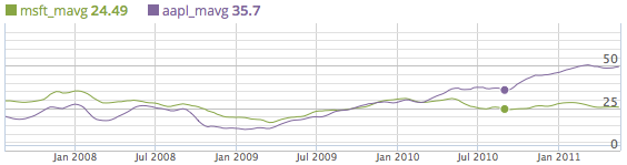
You can also pass variables as the series name using positional arguments. The value of the variable can change throughout the backtest, dynamically updating in the custom chart. The record function can accept a string or a variable that has a string value.
def initialize(context):
    # AA, AAPL, ALK
    context.securities = [sid(2), sid(24), sid(300)]

def handle_data(context, data):
    # You can pass a string variable into record().
    # Here we record the price of all the securities in our list.
    for stock in context.securities:
      price = data.current(stock, 'price')
      record(stock, price)

    # You can also pass in a variable with a string value.
    # This records the high and low values for AAPL.
    fields = ['high', 'low']
    for field in fields:
      record(field, data.current(sid(24),field))
The code produces a custom chart that looks like this. Click on a variable name in the legend to remove it from the chart, allowing you to zoom in on the other time series. Click the variable name again to restore it on the chart.
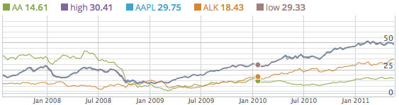
Some notes:
- For each series, the value at the end of each trading day becomes the recorded value for that day. This is important to remember when backtesting.
- Until a series starts being recorded, it will have no value. If
record(new_series=10)is done on day 10, new_series will have no value for days 1-9. - Each series will retain its last recorded value until a new value is used. If
record(my_series=5)is done on day 5, every subsequent day will have the same value (5) for my_series until a new value is given. - The backtest graph output automatically changes the x-axis time units when there are too many days to fit cleanly. For instance, instead of displaying 5 days of data individually, it will combine those into a 1-week data point. In that case the recorded values for that week are averaged and that average is displayed.
To see more, check out the example record algorithm at the end of the help documentation.
Dividends
The Quantopian database holds over 150,000 dividend events dating from January 2002. Dividends are treated as events and streamed through the performance tracking system that monitors your algorithm during a backtest. Dividend events modify the security price and the portfolio's cash balance.
In lookback windows, like history, prices are dividend-adjusted. Please review Data Sources for more detail.
Dividends specify four dates:
- declared date is the date on which the company announced the dividend.
- record date is the date on which a shareholder must be recorded as an owner to receive a dividend payment. Because settlement can take 3 days, a second date is used to calculate ownership on the record date.
- ex date is 3 trading days prior to the record date. If a holder sells the security before this date, they are not paid the dividend. The ex date is when the price of the security is typically most affected.
- pay date is the date on which a shareholder receives the cash for a dividend.
Security prices are marked down by the dividend amount on the open following the ex_date. The portfolio's cash position is increased by the amount of the dividend on the pay date. Quantopian chose this method so that cash positions are correctly maintained, which is particularly important when an algorithm is used for live trading. The downside to this method is that causes a lower portfolio value for the period between the two dates.
In order for your algorithm to receive dividend cash payments, you must have a long position (positive amount) in the security as of the close of market on the trading day prior to the ex_date AND you must run the simulation through the pay date, which is typically about 60 calendar days later.
If you are short the security at market close on the trading day prior to the ex_date, your algorithm will be required to pay the dividends due. As with long positions, the cash balance will be debited by the dividend payments on the pay date. This is to reflect the short seller's obligation to pay dividends to the entity that loaned the security.
Special dividends (where more than 25% of the value of the company is involved) are not yet tracked in Quantopian. There are several hundred of these over the last 11 years. We will add these dividends to our data in the future.
Dividends are not relayed to algorithms as events that can be accessed by the API; we will add that feature in the future.
Fundamental Data
Quantopian provides fundamental data from Morningstar, available in research and backtesting. The data covers over 8,000 companies traded in the US with over 900 metrics. Fundamental data can be accessed via the Pipeline API.
A full listing of the available fundamental fields can be found at the Fundamentals Reference page. Fundamental data is updated on a daily basis on Quantopian. A sample algorithm is available showing how to access fundamental data.
"as of" Dates
Each fundamental data field has a corresponding as_of field, e.g. shares_outstanding also has shares_outstanding_as_of. The as_of field contains the relevant time period of the metric, as a Python date object. Some of the data in Morningstar is quarterly (revenue, earnings, etc.), while other data is daily/weekly (market cap, P/E ratio, etc.). Each metric's as_of date field is set to the end date of the period to which the metric applies.
For example, if you use a quarterly earnings metric like shares_outstanding, the accompanying date field shares_outstanding_as_of will be set to the end date of the relevant quarter (for example, June 30, 2014). The as_of date indicates the date upon which the measured period ends.
Point in Time
When using fundamental data in Pipeline, Quantopian doesn't use the as_of date for exposing the data to your algorithm. Rather, a new value is exposed at the "point in time" in the past when the metric would be known to you. This day is called the file date.
Companies don't typically announce their earnings the day after the period is complete. If a company files earnings for the period ending June 30th (the as_of date), the file date (the date upon which this information is known to the public) is about 45 days later.
Quantopian takes care of this logic for you in both research and backtesting. For data updates since Quantopian began subscribing to Morningstar's data, Quantopian tracks the file date based on when the information changes in Morningstar. For historic changes, Morningstar also provides a file date to reconstruct how the data looked at specific points in time. In circumstances where the file date is not known to Quantopian, the file date is defaulted to be 45 days after the as_of date.
For a more technical explanation of how we store data in a "Point in Time" fashion, see this post in the community.
Setting a custom benchmark
The default benchmark in your algorithm is SPY, an ETF that tracks the S&P; 500. You can change it in the initialize function by using set_benchmark and passing in another security. Only one security can be used for the benchmark, and only one benchmark can be set per algorithm. If you set multiple benchmarks, the last one will be used. Currently, the benchmark can only be set to an equity.
Here's an example:
def initialize(context):
  set_benchmark(symbol('TSLA'))

def handle_data(context, data):
  ...
Slippage Models
Slippage is where our backtester calculates the realistic impact of your orders on the execution price you receive. When you place an order for a trade, your order affects the market. Your buy order drives prices up, and your sell order drives prices down; this is generally referred to as the 'price impact' of your trade. The size of the price impact is driven by how large your order is compared to the current trading volume. The slippage method also evaluates if your order is simply too big: you can't trade more than market's volume, and generally you can't expect to trade more than a fraction of the volume. All of these concepts are wrapped into the slippage method.
When an order isn't filled because of insufficient volume, it remains open to be filled in the next minute. This continues until the order is filled, cancelled, or the end of the day is reached when all orders are cancelled.
Slippage must be defined in the initialize method. It has no effect if defined elsewhere in your algorithm. To set slippage, use the set_slippage method and pass in FixedBasisPointsSlippage, FixedSlippage, VolumeShareSlippage, or a custom slippage model that you define.
def initialize(context):
    set_slippage(slippage.FixedBasisPointsSlippage(basis_points=5, volume_limit=0.1))
If you do not specify a slippage method, slippage for US equities defaults to the FixedBasisPointsSlippage model at 5 basis points fixed slippage. Futures follow a special volatility volume share model that uses 20-day annualized volatility as well as 20-day trading volume to model the price impact and fill rate of a trade. The model varies depending on which trading future and is explained in depth here. To set a custom slippage model for futures, pass a FixedSlippage model as a us_future keyword argument to set_slippage().
# Setting custom equity and futures slippage models.
def initialize(context):
    set_slippage(
        us_equities=slippage.FixedBasisPointsSlippage(basis_points=5, volume_limit=0.1),
        us_futures=slippage.FixedSlippage(spread=0)
    )
Fixed Basis Points Slippage
In the FixedBasisPointsSlippage model, the fill price of an order is a function of the order price, and a fixed percentage (in basis points). The basis_points constant (default 5) defines how large of an impact your order will have on the backtester's price calculation. The slippage is calculated by converting the basis_points constant to a percentage (5 basis points = 0.05%), and multiplying that percentage by the order price. Buys will fill at a price that is 0.05% higher than the close of the next minute, while sells will fill at a price that is 0.05% lower. A buy order for a stock currently selling at $100 per share would fill at $100.05 (100 + (0.0005 * 100)), while a sell order would fill at $99.95 (100 - (0.0005 * 100)).
The volume_limit cap (default 0.10) limits the proportion of volume that your order can take up per bar. For example: suppose you want to place an order, and 1000 shares trade in each of the next several minutes, and the volume_limit is 0.10. If you place an order for 220 shares then your trade order will be split into three transactions (100 shares, 100 shares, and 20 shares). Setting the volume_limit to 1.00 will permit the backtester to use up to 100% of the bar towards filling your order. Using the same example, this will fill 220 shares in the next minute bar.
Volume Share Slippage
In the VolumeShareSlippage model, the price you get is a function of your order size relative to the security's actual traded volume. You provide a volume_limit cap (default 0.025), which limits the proportion of volume that your order can take up per bar. For example: if the backtest is running in one-minute bars, and you place an order for 60 shares; then 1000 shares trade in each of the next several minute; and the volume_limit is 0.025; then your trade order will be split into three orders (25 shares, 25 shares, and 10 shares). Setting the volume_limit to 1.00 will permit the backtester to use up to 100% of the bar towards filling your order. Using the same example, this will fill 60 shares in the next minute bar.
The price impact constant (default 0.1) defines how large of an impact your order will have on the backtester's price calculation. The slippage is calculated by multiplying the price impact constant by the square of the ratio of the order to the total volume. In our previous example, for the 25-share orders, the price impact is .1 * (25/1000) * (25/1000), or 0.00625%. For the 10-share order, the price impact is .1 * (10/1000) * (10/1000), or .001%.
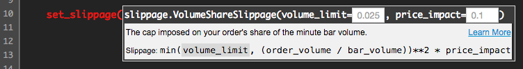
Fixed Slippage
When using the FixedSlippage model, the size of your order does not affect the price of your trade execution. You specify a 'spread' that you think is a typical bid/ask spread to use. When you place a buy order, half of the spread is added to the price; when you place a sell order, half of the spread is subtracted from the price.
Fills under fixed slippage models are not limited to the amount traded in the minute bar. In the first non-zero-volume bar, the order will be completely filled. This requires you to be careful about ordering; naive use of fixed slippage models will lead to unrealistic fills, particularly with large orders and/or illiquid securities.

Custom Slippage
You can build a custom slippage model that uses your own logic to convert a stream of orders into a stream of transactions. In the initialize() function you must specify the slippage model to be used and any special parameters that the slippage model will use. Example:
def initialize(context):
    set_slippage(MyCustomSlippage())
Your custom model must be a class that inherits from slippage.SlippageModel and implements process_order(self, data, order). The process_order method must return a tuple of (execution_price, execution_volume), which signifies the price and volume for the transaction that your model wants to generate. The transaction is then created for you.
Your model gets passed the same data object that is passed to your other functions, letting you do any price or history lookup for any security in your model. The order object contains the rest of the information you need, such as the asset, order size, and order type.
The order object has the following properties: amount (float), asset (Asset), stop and limit (float), and stop_reached and limit_reached (boolean). The trade_bar object is the same as data[sid] in handle_data and has open_price, close_price, high, low, volume, and sid.
The slippage.create_transaction method takes the given order, the data object, and the price and amount calculated by your slippage model, and returns the newly constructed transaction.
Many slippage models' behavior depends on how much of the total volume traded is being captured by the algorithm. You can use self.volume_for_bar to see how many shares of the current security have been traded so far during this bar. If your algorithm has many different orders for the same stock in the same bar, this is useful for making sure you don't take an unrealistically large fraction of the traded volume.
If your slippage model doesn't place a transaction for the full amount of the order, the order stays open with an updated amount value, and will be passed to process_order on the next bar. Orders that have limits that have not been reached will not be passed to process_order. Finally, if your transaction has 0 shares or more shares than the original order amount, an exception will be thrown.
Please see the sample custom slippage model.
Commission Models
To set the cost of your trades, use the set_commission method and pass in PerShare or PerTrade. Like the slippage model, set_commission must be used in the initialize method and has no effect if used elsewhere in your algorithm. If you don't specify a commission, your backtest defaults to $0.001 per share with a $0 minimum cost per trade.
def initialize(context):
    set_commission(commission.PerShare(cost=0.001, min_trade_cost=0))
Commissions are taken out of the algorithm's available cash. Regardless of what commission model you use, orders that are cancelled before any fills occur do not incur any commission.
The default commission model for US equities is PerShare, at $0.001 per share and $0 minimum cost per order. The first fill will incur at least the minimum commission, and subsequent fills will incur additional commission.
The PerTrade commission model applies a flat commission upon the first fill.
The default commission model for US futures is similar to retail brokerage pricing. Note that the model on Quantopian includes the $0.85 per contract commission that a broker might charge as well as the per-trade fees charged by the exchanges. The exchange fees vary per asset and are listed on this page under the heading "Exchange and Regulatory Fees".
To set a custom commission model for futures, pass a commission model as a us_future keyword argument to set_commission(). The available commission models for futures are a PerContract model that applies a cost and an exchange fee per contract traded, and a PerFutureTrade model that applies a cost per trade.
# Setting custom equity and futures commission models.
def initialize(context):
    set_commission(
        us_equities=commission.PerShare(cost=0.001, min_trade_cost=0),
        us_futures=commission.PerContract(cost=1, exchange_fee=0.85, min_trade_cost=0)
    )
You can see how much commission has been associated with an order by fetching the order using get_order and then looking at its commission field.
Self-Serve Data
Self-Serve Data provides you the ability to upload your own time-series data to Quantopian and access it in research and the IDE directly via Pipeline. You can add historical data as well as live-updating data on a nightly basis.
Important Concepts
Your custom data will be processed similar to Quantopian Partner Data. In order to accurately represent your data in pipeline and avoid lookahead bias, your data will be collected, stored, and surfaced in a point-in-time nature. You can learn more about our process for working with point-in-time data here: How is it Collected, Processed, and Surfaced? . A more detailed description, Three Dimensional Time Working with Alternative Data, is also available.
Once on the platform, your datasets are only importable and visible by you. If you share an algorithm or notebook that uses one of your private datasets, other community members won't be able to import the dataset. Your dataset will be downloaded and stored on Quantopian maintained servers where it is encrypted at rest.
Dataset Upload Format
Initially, this feature supports reduced custom datasets that have a single row of data per asset per day in csv file format . This format fits naturally into the expected pipeline format.
Two Data Column CSV Example
Below is a very simple example of a .csv file that can be uploaded to Quantopian. The first row of the file must be a header, and columns are separated by the comma character (,).
date,symbol,signal1,signal2
2014-01-01,TIF,1204.5,0
2014-01-02,TIF,1225,0.5
2014-01-03,TIF,1234.5,0
2014-01-06,TIF,1246.3,0.5
2014-01-07,TIF,1227.5,0
Data Columns
Data should be in csv format (comma-separated value) with a minimum of three columns: one primary date, one primary asset and one or more value columns.
Note: Column Names must be unique and contain only alpha-numeric characters and underscores.
-
Primary Date: A column must be selected as the primary date - A date column to which the record's values apply, generally it’s the day on which you learned about the information. You may also know this as the primary date or the asof_date for other items in the Quantopian universe. Data before 2002 will be ignored. Blank or NaN/NaT values will cause errors
Example Date Formats:
2018-01-01, 20180101, 01/01/2018, 1/1/2018. Note: datetimeasof_datevalues are not supported in our existing pipeline extraction, please contact us at [email protected] to discuss your use case. -
Primary Asset: A column must be selected as the primary asset. This symbol column is used to identify assets on that date. If you have multiple share classes of an asset, those should be identified on the symbol with a delimiter (-,/,.,_). ex: "BRK_A" or "BRK/A"
Note: Blank values will cause errors. Records that cannot be mapped from symbols to assets in the Quantopian US equities database will be skipped
-
Value(s) (1+): One or more value columns provided by the user for use in their particular strategy. The example .csv file earlier in this document has 2 value columns.
During the historical upload process, you will need to map your data columns into one of the acceptable data formats below:
- Numeric- Values. Note that these will be converted to floats to maximize precision in future calculation.
- String- Textual values which do not need further conversion. Often titles, or categories.
- Date- This will not be used as the primary date column, but can still be examined within the algorithm or notebook. Date type columns are not adjusted during Timezone adjustment. Example Date Formats:
2018-01-01, 20180101, 01/01/2018, 1/1/2018 - Datetime- Date with a timestamp (in UTC), values will be adjusted when the incoming Timezone is configured to a value other than UTC. A general datetime field that can be examined within the algorithm or notebook. Example DateTime Formats:
[Sample Date] 1:23or[Sample Date] 20:23-05:00(with timezone designator) - Bool- True or False values (0,'f','F','false','False','FALSE' and 1,'t','T','true','True','TRUE')
- Reserved Column Names: timestamp and sid will be added by Quantopian during data processing, you cannot use these column names in your source data. If you have a source column named symbol, it must be set as the Primary Asset.
- NaN values: By default the following values will be interpreted as NaN: '', '#N/A', '#NA', 'N/A', '-NaN', 'NULL', 'NaN', 'null'
- Infinite values: By default 'inf' or '-inf' values will be interpreted as positive and negative infinite values.
Uploading Your Data
Uploading your data is done in 1 or 2 steps. The first step is an upload of historical data, and the (optional) second step is to set up the continuous upload of live data.
When uploading your historical data to Quantopian you will be required to declare each column type. Once the column types have been declared we will validate that all the historical data can be processed.
Important Date Assumptions
When surfacing alternative data in pipeline, Quantopian makes assumptions based on a common data processing workflow for dataset providers. Typically data is analyzed after market close and is stamped as a value as of that day. Since the data was not available for the full trading day, it will only be surfaced in pipeline the next trading day.
- Asof_date - This is mapped to the primary date column.
Asof_datewill be surfaced the next trading day in pipeline. Ex: an asof_date on 02/14/2018 (timestamp 2018-02-15 07:12:03.6) will be surfaced in pipeline on 02/15/2018 - Timestamp - This is a date generated by Quantopian that is the datetime at which the Quantopian system learns about a particular data point (knowledge datetime). For live data, it is inferred by the Quantopian data system based on when it reads the data from the FTP or URL.
Preparing your historical data:
During the historical upload, Quantopian will translate the primary date column values into a historical timestamp by adding a historical lag (default: one day).
In the example above, the date column was selected as the primary date and adjusted to create the historical timestamps.

Corner cases to think about:
- Avoid lookahead data: The
primary datecolumn should not include future dated historical values, we will ignore them. A similar requirement exists for live data, theasof_datemust not be greater than thetimestamp. Note: These will cause issues with pipeline. - Trade Date Signals: If your date field represents the day you expect an algorithm to act on the signal, you should create a
trade_date_minus_onecolumn that can be used as the primary date column.
Adding Your Dataset
Navigate to the account page data tab and click Add Dataset under the Self-Serve Data section.
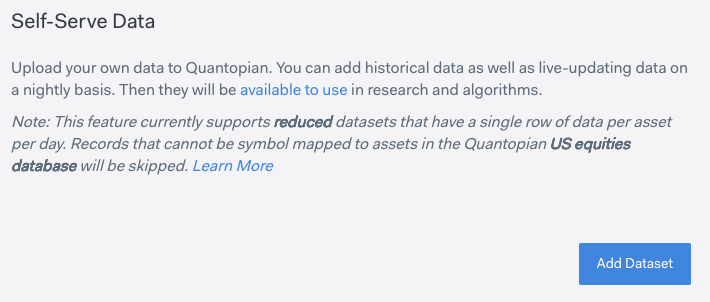
Name Your Dataset
Dataset Name: Used as namespace for importing your dataset. The name must start with a letter and must contain only lowercase alpha-numeric and underscore characters.
Upload and Map Historical Data
Click or drag a file to upload into the historical data drag target. Clicking on the button will bring up your computer’s file browser.
Once a file has been successfully loaded in the preview pane, you must define one Primary Date and one Primary Asset column and map all of the data columns to specific types.

Configure Historical Lag
Historical timestamps are generated by adding the historical lag to the primary date. The default historical lag is one day, which will prevent end of day date type values from appearing in pipeline a day early. ex: 2018-03-02 with a one hour lag would create a historical timestamp of 2018-03-02 01:00:00, which would incorrectly appear in pipeline on 2018-03-02. The default one day historical lag adjusts them to appear correctly in pipeline on 2018-03-03.
Configure Timezone
By default, datetime values are expected in UTC or should include a timezone designator. If another timezone is selected (ex: US/Eastern), the incoming datetime type columns will be converted to UTC when a timezone designator is not provided. ex: Note: date type columns will not be timezone adjusted.
Be careful when determining the timezone of a new datasource with datetime values that don't have the timezone designator. For example, GOOGLEFINANCE in Google Sheets returns dates like YYYY-MM-DD 16:00:00, which are end-of-day values for the market in East Coast time. Selecting US/Eastern will properly convert the datetime to YYYY-MM-DD 20:00:00 during daylight savings time and YYYY-MM-DD 21:00:00 otherwise.
Selecting Next will complete the upload and start the data validation process.
Set Up Live Data
Once your historical data has successfully validated, you’ll navigate to the Set Up Live Data tab.
You can configure your Connection Type settings to download a new file daily. In addition to the standard FTP option, live data can be downloaded from hosted CSV files like Google Sheets, Dropbox or any API service that supports token-based urls (vs authentication).
Each trading day, between 07 to 10 am UTC, this live file will be downloaded and compared against existing dataset records. Brand new records will be added to the base tables and updates will be added to the deltas table based on the Partner Data process logic.
Note: Column names must be identical between the historical and live files. The live data download will use the same column types as configured during the historical upload.
Clicking submit will add your dataset to the historical dataset ingestion queue. You can navigate to your specific dataset page by clicking on the Dataset name in the Self-Serve Data section. This page is only viewable to you and includes the First Load Date, and code samples for pipeline use.
From Google Sheets
You can import a CSV from your Google Sheets spreadsheet. To get the public URL for your file:
- Click on File > Publish to the web.
- Change the 'web page' option to 'comma-separated values (.csv)'.
- Click the Publish button.
- Copy and paste the URL that has a format similar to
https://docs.google.com/spreadsheets/d/e/2PACX-1vQqUUOUysf9ETCvRCZS8EGnFRc4k7yd8IUshkNyfFn2NEeuCGNBFXfkXxyZr9HOYQj34VDp_GWlX_NX/pub?gid=1739886979&single;=true&output;=csv.
Google Sheets has powerful IMPORTDATA and QUERY functions that can be used to download API data, rename columns and filter by columns/dates etc in an automatic fashion. QUERY(Sample!A1:L,"select A,K,L,D,E,B,G,H WHERE A >= date '2018-03-01'")
From Dropbox
To use Dropbox, place your file in the Public folder and use the 'Public URL'. The Public URL has a format similar to https://dl.dropboxusercontent.com/s/1234567/filename.csv.
Historical Dataset Ingestion
The typical delay from dataset submission to full availability is approximately 15 minutes. You can monitor the status by checking the load_metrics data in research.
Accessing Your Dataset
Private datasets are accessible via pipeline in notebooks and algorithms. Interactive datasets and deltas are also available in research.
Research Notebooks
If you are a loading a new dataset into a notebook you will need to Restart to be able to access the new import. The dataset can be imported before all the data is fully available.
You can monitor the status by checking the load_metrics data in research. This will also help you identify any rows that were skipped during the upload (trim before 2002-01-01) and symbol mapping process (rows_received - total_rows).
from odo import odo
from quantopian.interactive.data.user_<UserId> import load_metrics
lm = odo(load_metrics[['timestamp','dataset','status','rows_received','total_rows'
                    ,'rows_added','delta_rows_added','last_updated','time_elapsed'
                    ,'filenames_downloaded','source_last_updated','bytes_downloaded'
                    ,'db_table_size','error'
                   ]].sort('timestamp',ascending=False), pd.DataFrame)
lm
Research Pipeline
Clicking on the dataset link on the Self-Serve Data section will take you to a page with a How to Use example that shows you how to setup the full pipeline.
Research Interactive
You will also be able to look at the raw upload via the interactive version
 from quantopian.interactive.data.<UserId> import <dataset> as dataset
 print len(dataset)
 dataset.dshape
If live loads are configured, you may start to see adjustment records appearing in the deltas table
 from quantopian.interactive.data.<UserId> import <dataset>_deltas as datasetd
 datasetd['timestamp'].max()
In Algorithm Use
The pipeline dataset is the method of accessing your data in algorithms
from quantopian.pipeline.data.<UserId> import <dataset> as my_dataset
The example long short equity algorithm lecture is a good example that leverages a publicly available dataset.
You'll want to replace the following stocktwits import with your specific dataset and then update or replace the sentiment_score with a reference to your dataset column (adjusting the SimpleMovingAverage factor as needed).
 from quantopian.pipeline.data.psychsignal import stocktwits

    sentiment_score = SimpleMovingAverage(
        inputs=[stocktwits.bull_minus_bear],
        window_length=3,
    )
Monitoring DataSet Loads
We have surfaced an interactive load_metrics dataset that will allow you to easily monitor the details and status of your dataset historical loads and daily live updates.
 from odo import odo
 from quantopian.interactive.data.user_<UserId> import load_metrics
 lm = odo(load_metrics[['timestamp','dataset','status','rows_received','total_rows'
                       ,'rows_added','delta_rows_added','last_updated','time_elapsed'
                       ,'filenames_downloaded','source_last_updated','bytes_downloaded'
                       ,'db_table_size','error'
                      ]].sort('timestamp',ascending=False), pd.DataFrame)
lm- filenames_downloaded: name(s) of the files that were downloaded
- rows_received: Total number of raw rows downloaded from historical or ftp
- rows_added: Number of new records added to base dataset table (after symbol mapping and deduping by asset/per day)
- total_rows: Total number of rows in the base table after the load completed
- delta_rows_added: Number of new records added to the deltas (updates) table
- total_delta_rows: Total number of rows in the deltas table after the load completed
- timestamp: start time of the download
- time_elapsed: Number of seconds it took to process the data
- last_updated: (live loads) the maximum timestamp for records added to the base table (Historical) the timestamp of historical load completion
- source_last_updated: file timestamp on the source ftp file (live loads only)
- status: [running, empty (no data to process), failed, completed]
- error: error message for failed runs
Dataset Limits
- Initial limit of 30 datasets (Note: currently datasets cannot be modified after submission)
- Maximum of 20 columns
- Maximum file size of 300MB
- Maximum dataset name of 56 characters
- Live uploads will be processed on trading days from 07 to 10 am UTC
You can still load static historical data to research with local_csv, or to an algorithm with fetch_csv, but the data cannot be added to Pipeline in either scenario.
Fetcher - Load any CSV file
Note: The best way to upload a time-series csv, with accurate point-in-time data via Pipeline, is the Self-Serve data feature. Fetcher should not be used in algorithms attempting to enter the contest or receive an investment allocation.
Quantopian provides historical data since 2002 for US equities in minute bars. The US market data provides a backbone for financial analysis, but some of the most promising areas of research are finding signals in non-market data. Fetcher provides your algorithm with access to external time series data. Any time series that can be retrieved as a CSV file via http or https can be incorporated into a Quantopian algorithm.
Fetcher lets Quantopian download CSV files and use them in your simulations. To use it, use fetch_csv(url) in your initialize method. fetch_csv will download the CSV file and parse it into a pandas dataframe. You may then specify your own methods to modify the entire dataframe prior to the start of the simulation. During simulation, the rows of the CSV/dataframe are provided to your algorithm's handle_data and other functions as additional properties of the data parameter.
Best of all, your Fetcher data will play nicely with Quantopian's other data features:
- Use
recordto plot a time series of your fetcher data. - Your data will be streamed to your algorithm without look-ahead bias. That means if your backtest is currently at 10/01/2013 but your Fetcher data begins on 10/02/2013, your algorithm will not have access to the Fetcher data until 10/02/2013. You can account for this by checking the existence of your Fetcher field, see common errors for more information.
Fetcher supports two kinds of time series:
- Security Information: data that is about individual securities, such as short interest for a stock
- Signals: data that stands alone, such as the Consumer Price Index, or the spot price of palladium
For Security Info, your CSV file must have a column with header of 'symbol' which represents the symbol of that security on the date of that row. Internally, Fetcher maps the symbol to the Quantopian security id (sid). You can have many securities in a single CSV file. To access your CSV data in handle_data:
## This algo imports sample short interest data from a CSV file for one security,
## NFLX, and plots the short interest:

def initialize(context):
    # fetch data from a CSV file somewhere on the web.
    # Note that one of the columns must be named 'symbol' for
    # the data to be matched to the stock symbol
    fetch_csv('https://dl.dropboxusercontent.com/u/169032081/fetcher_sample_file.csv',
               date_column = 'Settlement Date',
               date_format = '%m/%d/%y')
    context.stock = symbol('NFLX')

def handle_data(context, data):
    record(Short_Interest = data.current(context.stock, 'Days To Cover'))
Here is the sample CSV file. Note that for the Security Info type of import, one of the columns must be 'symbol'.
Settlement Date,symbol,Days To Cover
9/30/13,NFLX,2.64484
9/13/13,NFLX,2.550829
8/30/13,NFLX,2.502331
8/15/13,NFLX,2.811858
7/31/13,NFLX,1.690317
For Signals, your CSV file does not need a symbol column. Instead, you provide it via the symbol parameter:
def initialize(context):
    fetch_csv('https://yourserver.com/cpi.csv', symbol='cpi')

def handle_data(context, data):
    # get the cpi for this date
    current_cpi = data.current('cpi','value')

    # plot it
    record(cpi=current_cpi)
Importing Files from Dropbox
Many users find Dropbox to be a convenient way to access CSV files. To use Dropbox, place your file in the Public folder and use the 'Public URL'. A common mistake is to use a URL of format https://www.dropbox.com/s/abcdefg/filename.csv, which is a URL about the file, not the file itself. Instead, you should use the Public URL which has a format similar to https://dl.dropboxusercontent.com/u/1234567/filename.csv.
Importing Files from Google Drive
If you don't have a public Dropbox folder, you can also import a CSV from your Google Drive. To get the public URL for your file:
- Click on File > Publish to the web.
- Change the 'web page' option to 'comma-separated values (.csv)'.
- Click the Publish button.
- Copy and paste the URL into your Fetcher query.
Data Manipulation with Fetcher
If you produce the CSV, it is relatively easy to put the data into a good format for Fetcher. First decide if your file should be a signal or security info source, then build your columns accordingly.
However, you may not always have control over the CSV data file. It may be maintained by someone else, or you may be using a service that dynamically generates the CSV. Quandl, for example, provides a REST API to access many curated datasets as CSV. While you could download the CSV files and modify them before using them in Fetcher, you would lose the benefit of the nightly data updates. In most cases it's better to request fresh files directly from the source.
Fetcher provides two ways to alter the CSV file:
pre_funcspecifies the method you want to run on the pandas dataframe containing the CSV immediately after it was fetched from the remote server. Your method can rename columns, reformat dates, slice or select data - it just has to return a dataframe.post_funcis called after Fetcher has sorted the data based on your given date column. This method is intended for time series calculations you want to do on the entire dataset, such as timeshifting, calculating rolling statistics, or adding derived columns to your dataframe. Again, your method should take a dataframe and return a dataframe.
Live Trading and Fetcher
When Fetcher is used in Live Trading or Paper Trading, the fetch_csv() command is invoked once per trading day, when the algorithm warms up, before market open. It's important that the fetched data with dates in the past be maintained so that warm up can be performed properly; Quantopian does not keep a copy of your fetched data, and algorithm warmup will not work properly if past data is changed or removed. Data for 'today' and dates going forward can be added and updated.
Any updates to the CSV file should happen before midnight Eastern Time for the data to be ready for the next trading day.
Working With Multiple Data Frequencies
When pulling in external data, you need to be careful about the data frequency to prevent look-ahead bias. All Quantopian backtests are run on minutely frequency. If you are fetching daily data, the daily row will be fetched at the beginning of the day, instead of the end of day. To guard against the bias, you need to use the post_func function. For more information see post_func API documentation or take a look at this example algorithm.
History() is not supported on fetched data. For a workaround, see this community forum post.
For more information about Fetcher, go to the API documentation or look at the sample algorithms.
Figuring out what assets came from Fetcher
It can be useful to know which assets currently have Fetcher signals for a given day. data.fetcher_assets returns a list of assets that, for the given backtest or live trading day, are active from your Fetcher file.
Here's an example file with ranked securities:
symbol, start date, stock_score
AA,     2/13/12,     11.7
WFM,    2/13/12,     15.8
FDX,    2/14/12,     12.1
M,      2/16/12,     14.3
You can backtest the code below during the dates 2/13/2012 - 2/18/2012. When you use this sample file and algorithm, data.fetcher_assets will return, for each day:
- 2/13/2012: AA, WFM
- 2/14/2012: FDX
- 2/15/2012: FDX (forward filled because no new data became available)
- 2/16/2012: M
Note that when using this feature in live trading, it is important that all historical data in your fetched data be accessible and unchanged. We do not keep a copy of fetched data; it is reloaded at the start of every trading day. If historical data in the fetched file is altered or removed, the algorithm will not run properly. New data should always be appended to (not overwritten over) your existing Fetcher .csv source file. In addition, appended rows cannot contain dates in the past. For example, on May 3rd, 2015, a row with the date May 2nd, 2015, could not be appended in live trading.
Validation
Our IDE has extensive syntax and validation checks. It makes sure your algorithm is valid Python, fulfills our API, and has no obvious runtime exceptions (such as dividing by zero). You can run the validation checks by clicking on the Build button (or pressing control-B), and we'll run them automatically right before starting a new backtest.
Errors and warnings are shown in the window on the right side of the IDE. Here's an example where the log line is missing an end quote.

When all errors and warnings are resolved, the Build button kicks off a quick backtest. The quick backtest is a way to make sure that the algorithm roughly does what you want it to, without any errors.
Once the algorithm is running roughly the way you'd like, click the 'Full Backtest' button to kick off a full backtest with minute-bar data.
Module Import
Only specific, whitelisted portions of Python modules can be imported. Select portions of the following libraries are allowed. If you need a module that isn't on this list, please let us know.
bisectblazecmathcollectionscopycvxoptcvxpydatetimefunctoolsheapqitertoolsmathnumpyodooperatorpandaspykalmanpytzquantopianQueuerescipysklearnsqlalchemystatsmodelstalibtimeziplinezlib
Collaboration
You can collaborate in real-time with other Quantopian members on your algorithm. In the IDE, press the “Collaborate” button and enter your friend’s email address. Your collaborators will receive an email letting them know they have been invited. They will also see your algorithm listed in their Algorithms Library with a collaboration icon. If your collaborator isn't yet a member of Quantopian, they will have to register before they can see your algorithm.

The collab experience is fully coordinated:
- The code is changed on all screens in real time.
- When one collaborator "Builds" a backtest, all of the collaborators see the backtest results, logging, and/or errors.
- There is a chat tab for you to use while you collaborate.
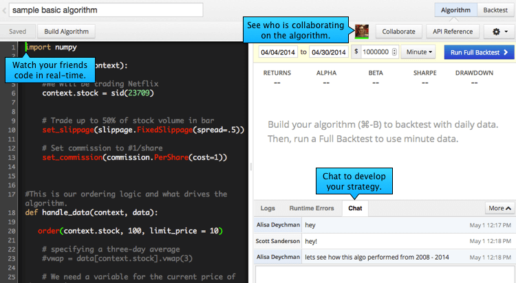
Technical Details
- Only the owner can invite other collaborators, deploy the algorithm for live trading, or delete the algorithm.
- There isn't a technical limit on number of collaborators, but there is a practical limit. The more collaborators you have, the more likely that you'll notice a performance problem. We'll improve that in the future.
- To connect with a member, search their profile in the forums and send them a private message. If they choose to share their email address with you, then you can invite them to collaborate.
Futures
There are a number of API functions specific to futures that make it easy to get data or trade futures contracts in your algorithms. A walkthrough of these tools is available in the Futures Tutorial.
Continuous Futures
Futures contracts have short lifespans. They traded for a specific period of time before they expire at a pre-determined date of delivery. In order to hold a position over many days in an underlying asset, you might need to close your position in an expiring contract and open a position in the next contract. Similarly, when looking back at historical data, you need to get pricing or volume data from multiple contracts to get a series of data that reflects the underlying asset. Both of these problems can be solved by using continuous futures.
Continuous futures can be created with the continuous_future function. Using the continuous_future function brings up a search box for you to look up the root symbol of a particular future.
Continuous futures are abstractions over the 'underlying' commodities/assets/indexes of futures. For example, if we wanted to trade crude oil, we could create a reference to CL, instead of a list of CLF16, CLG16, CLH16, CLJ16, etc.. Instead of trying to figure out which contract in the list we want to trade on a particular date, we can use the continuous future to get the current active contract. We can do this by using using data.current() as shown in this example:
def initialize(context):
    # S&P; 500 E-Mini Continuous Future
    context.future = continuous_future('ES')
    schedule_function(daily_func, date_rules.every_day(), time_rules.market_open())

def daily_func(context, data):
    es_active = data.current(context.future, 'contract')
It is important to understand that continuous futures are not tradable assets. They simply maintain a reference to the active contracts of an underlying asset, so we need to get the underlying contract before placing an order.
Continuous futures allow you to maintain a continuous reference to an underlying asset. This is done by stitching together consecutive contracts. This plot shows the volume history of the crude oil continuous future as well as the volume of the individual crude oil contracts. As you can see, the volume of the continuous future is the skyline of the contracts that make it up.

Historical Data Lookup
Continuous futures make it easy to look up the historical price or volume data of a future, without having to think about the individual contracts underneath it. To get the history of a future, you can simply pass a continuous future as the first argument to data.history().
def initialize(context):
    # S&P; 500 E-Mini Continuous Future
    context.future = continuous_future('ES')
    schedule_function(daily_func, date_rules.every_day(), time_rules.market_open())

def daily_func(context, data):
    es_history = data.history(context.future, fields='price', bar_count=5, frequency='1d')
Daily frequency history is built on 24 hour trade data. A daily bar for US futures captures the trade activity from 6pm on the previous day to 6pm on the current day (Eastern Time). For example, the Monday daily bar captures trade activity from 6pm the day before (Sunday) to 6pm on the Monday. Tuesday's daily bar will run from 6pm Monday to 6pm Tuesday, etc. Minute data runs 24 hours and is available from 6pm Sunday to 6pm Friday each week.
In general, there is a price difference between consecutive contracts for the same underlying asset/commodity at a given point in time. This difference is caused by the opportunity cost and the carry cost of holding the underlying asset for a longer period of time. For example, the storage cost of holding 1000 barrels of oil might push the cost of a contract with delivery in a year to be higher than the cost of a contract with delivery in a month - the cost of storing them for a year would be significant. These price differences tend not to represent differences in the value of the underlying asset or commodity. To factor these costs out of a historical series of pricing data, we make an adjustment on a continuous future. The adjustment removes the difference in cost between consecutive contracts when the continuous future is stitched together. By default, the price history of a continuous future is adjusted. Prices are adjusted backwards from the current simulation date in a backtest. By using adjusted prices, you can make meaningful computations on a continuous price series.
The following plot shows the adjusted price of the crude oil continuous future. It also shows the prices of the individual 'active' contracts underneath. The adjusted price factors out the jump between each pair of consecutive contracts.

The adjustment method can be specified as an argument to the continuous_future function. This can either be set to adjustment='add' which subtracts the difference in consecutive contract prices from the historical series, or 'mul' which multiplies out the ratio between consecutive contracts. The 'mul' technique is the default used on Quantopian.
The continuous_future function also takes other optional arguments.
The offset argument allows you to specify whether you want to maintain a reference to the front contract or to a back contract. Setting offset=0 (default) maintains a reference to the front contract, or the contract with the next soonest delivery. Setting offset=1 creates a continuous reference to the contract with the second closest date of delivery, etc.
The roll argument allows you to specify the method for determining when the continuous future should start pointing to the next contract. By setting roll='calendar', the continuous future will start pointing to the next contract as the 'active' one when it reaches the auto_close_date of the current contract. By setting roll='volume', the continuous future will start pointing to the next contract as the 'active' one when the volume of the next contract surpasses the volume of the current active contract, as long as it's withing 7 days of the auto_close_date of the current contract.
The following code snippet creates a continuous future for the front contract, using the calendar roll method, to be adjusted using the 'mul' technique when making historical data requests.
def initialize(context):
    # S&P; 500 E-Mini Continuous Future
    context.future = continuous_future('ES', offset=0, roll='calendar', adjustment='mul')
Continuous futures are explained further in the Futures Tutorial.
Upcoming Contract Chain
Sometimes, knowing the forward looking chain of contracts associated with a particular future can be helpful. For example, if you want to trade back contracts, you will need to reference contracts with delivery dates several months into the future. This can be done with the data.current_chain() function.
def initialize(context):
    # Crude Oil Continuous Future
    context.future = continuous_future('CL')
    schedule_function(daily_func, date_rules.every_day(), time_rules.market_open())

def daily_func(context, data):
    cl_chain = data.current_chain(context.future)
    front_contract = cl_chain[0]
    secondary_contract = cl_chain[1]
    tertiary_contract = cl_chain[2]
Available Futures
Below is a list of futures that are currently available on Quantopian. Note that some of these futures may no longer be trading but are included in research and backtesting to avoid forward lookahead bias. The data for some futures in the Quantopian database starts after 2002. This visualization shows the start and end of the data we have for each future.
|
Name
|
Root Symbol
|
Exchange
|
|---|---|---|
| Soybean Oil | BO | CBOT |
| Corn E-Mini | CM | CBOT |
| Corn | CN | CBOT |
| Ethanol | ET | CBOT |
| 30-Day Federal Funds | FF | CBOT |
| 5-Year Deliverable Interest Rate Swap Futures | FI | CBOT |
| TNote 5 yr | FV | CBOT |
| Soybeans E-Mini | MS | CBOT |
| Wheat E-Mini | MW | CBOT |
| Oats | OA | CBOT |
| Rough Rice | RR | CBOT |
| Soybean Meal | SM | CBOT |
| Soybeans | SY | CBOT |
| 10-Year Deliverable Interest Rate Swap Futures | TN | CBOT |
| TNote 2 yr | TU | CBOT |
| TNote 10 yr | TY | CBOT |
| Ultra Tbond | UB | CBOT |
| TBond 30 yr | US | CBOT |
| Wheat | WC | CBOT |
| Dow Jones E-mini | YM | CBOT |
| Big Dow | BD | CBOT (no longer trading) |
| DJIA Futures | DJ | CBOT (no longer trading) |
| 5-Year Interest Rate Swap Futures | FS | CBOT (no longer trading) |
| Municipal Bonds | MB | CBOT (no longer trading) |
| 10-Year Interest Rate Swap Futures | TS | CBOT (no longer trading) |
| VIX Futures | VX | CFE |
| Australian Dollar | AD | CME |
| Bloomberg Commodity Index Futures | AI | CME |
| British Pound | BP | CME |
| Canadian Dollar | CD | CME |
| Euro FX | EC | CME |
| Eurodollar | ED | CME |
| Euro FX E-mini | EE | CME |
| S&P 500 E-Mini | ES | CME |
| E-micro EUR/USD Futures | EU | CME |
| Feeder Cattle | FC | CME |
| Japanese Yen E-mini | JE | CME |
| Japanese Yen | JY | CME |
| Lumber | LB | CME |
| Live Cattle | LC | CME |
| Lean Hogs | LH | CME |
| Mexican Peso | ME | CME |
| S&P 400 MidCap E-Mini | MI | CME |
| Nikkei 225 Futures | NK | CME |
| NASDAQ 100 E-Mini | NQ | CME |
| New Zealand Dollar | NZ | CME |
| Swiss Franc | SF | CME |
| S&P 500 Futures | SP | CME |
| S&P 400 MidCap Futures | MD | CME (no longer trading) |
| NASDAQ 100 Futures | ND | CME (no longer trading) |
| Pork Bellies | PB | CME (no longer trading) |
| TBills | TB | CME (no longer trading) |
| Gold | GC | COMEX |
| Copper High Grade | HG | COMEX |
| Silver | SV | COMEX |
| NYSE Comp Futures | YX | NYFE |
| Light Sweet Crude Oil | CL | NYMEX |
| NY Harbor USLD Futures (Heating Oil) | HO | NYMEX |
| Natural Gas | NG | NYMEX |
| Palladium | PA | NYMEX |
| Platinum | PL | NYMEX |
| Natural Gas E-mini | QG | NYMEX |
| Crude Oil E-Mini | QM | NYMEX |
| RBOB Gasoline Futures | XB | NYMEX |
| Unleaded Gasoline | HU | NYMEX (no longer trading) |
| MSCI Emerging Markets Mini | EI | ICE |
| MSCI EAFE Mini | MG | ICE |
| Gold mini-sized | XG | ICE |
| Silver mini-sized | YS | ICE |
| Sugar #11 | SB | ICE |
| Russell 1000 Mini | RM | ICE |
| Russell 2000 Mini | ER | ICE |
| Eurodollar | EL | ICE (no longer trading) |
Running Backtests
You can set the start date, end date, starting capital, and trading calendar used by the backtest in the IDE.

SPY, an ETF tracking the S&P; 500, is the benchmark used for algorithms simulated in the backtest. It represents the total returns and reinvests the dividends to model the market performance. You can also set your own benchmark in your algorithm.
To create a new backtest, click the 'Run Full Backtest' button from the IDE. That button appears once your algorithm successfully validates. Press the 'Build' button to start the validation if the 'Run Full Backtest' button is not visible in the upper-right of the IDE.
We also provide a Backtests Page that has a summary of all backtests run against an algorithm. To go to the Backtests page, either click the Backtest button at the top right of the IDE, or, from the My Algorithms page click the number of backtests that have been run. The backtests page lists all the backtests that have been run for this algorithm, including any that are in progress. You can view an existing or in-progress backtest by clicking on it. Closing the browser will not stop the backtest from running. Quantopian runs in the cloud and it will continue to execute your backtest until it finishes running. If you want to stop the backtest, press the Cancel button.
Debugger
The debugger gives you a powerful way to inspect the details of a running backtest. By setting breakpoints, you can pause execution and examine variables, order state, positions, and anything else your backtest is doing.
Using the Debugger
In the IDE, click on a line number in the gutter to set a breakpoint. A breakpoint can be set on any line except comments and method definitions. A blue marker appears once the breakpoint is set.
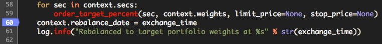
To set a conditional breakpoint, right-click on a breakpoint's blue marker and click 'Edit Breakpoint'. Put in some Python code and the breakpoint will hit when this condition evaluates to true. In the example below, this breakpoint hits when the price of Apple is above $100. Conditional breakpoints are shown in yellow in the left-hand gutter.
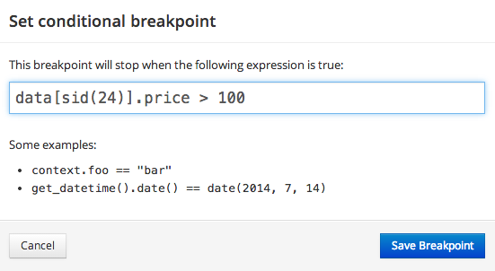
You can set an unlimited number of breakpoints. Once the backtest has started, it will stop when execution gets to a line that has a breakpoint, at which point the backtest is paused and the debug window is shown. In the debugger, you can then query your variables, orders and portfolio state, data, and anything else used in your backtest. While the debugger window is active, you can set and remove other breakpoints.
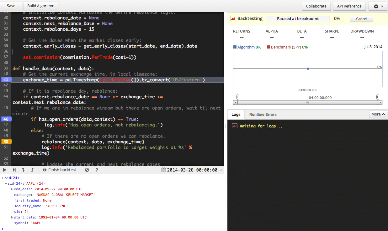
To inspect an object, enter it in the debug window and press enter. Most objects will be pretty-printed into a tree format to enable easy inspection and exploration.
The following commands can be used in the debugger window:
| Keyboard Shortcut | Action |
| .c or .continue | Resume backtest until it triggers the next breakpoint or an exception is raised. |
| .n or .next | Executes the next line of code. This steps over the next expression. |
| .s or .step | Executes the next line of code. This steps into the next expression, following function calls. |
| .r or .return | Execute until you are about to return from the current function call. |
| .f or .finish | Disables all breakpoints and finishes the backtest. |
| .clear | Clears the data in the debugger window. |
| .h or .help | Shows the command shortcuts for the debugger. |
Technical Details
- The debugger is available in the IDE. It is not available on the Full Backtest screen.
- You can edit your code during a debugging session, but those edits aren't used in the debugger until a new backtest is started.
- After 10 minutes of inactivity in the IDE, any breakpoints will be suspended and the backtest will automatically finish running.
- After 50 seconds, the breakpoint commands will timeout. This is the same amount of time given for 1 handle_data call.
Backtest results
Once a full backtest starts, we load all the trading events for the securities that your algorithm specified, and feed them to your algorithm in time order. Results will start streaming in momentarily after the backtest starts.
Here is a snapshot of a backtest results page. Mouse over each section to learn more.

Backtest settings and status: Shows the initial settings for the backtest, the progress bar when the backtest is in progress, and the final state once the test is done. If the backtest is cancelled, exceeds its max daily loss, or have runtime errors, that information will be displayed here.
Result details: Here's where you dive into the details of your backtest results. You can examine every transaction that occurred during the backtest, see how your positions evolved over time, and look at detailed risk metrics. For the risk metrics, we show you 1, 3, 6, and 12-month windows to provide more granular breakdowns
Overall results: This is the overall performance and risk measures of your backtest. These numbers will update during the course of the backtest as new data comes in.
Cumulative performance and benchmark overlay: Shows your algorithm's performance over time (in blue) overlaid with the benchmark (in red).
Daily and weekly P/L: Shows your P/L per day or week, depending on the date range selected.
Transactions chart: Shows all the cumulative dollar value of all the buys and sells your algorithm placed, per day or week. Buys are shown as positive blue, and sells as negative reds.
Trading Guards
There are several trading guards you can place in your algorithm to prevent unexpected behavior. All the guards are enforced when orders are placed. These guards are set in the initialize function.
Set Restrictions On Specific Assets
You can prevent the algorithm from trading specific assets by using set_asset_restrictions. If the algorithm attempts to order any asset that is restricted, it will stop trading and throw an exception. To avoid attempts to order any restricted assets, use the can_trade method, which will return False for assets that are restricted at that point in time.
We've built a point-in-time asset restriction for you that includes all the leveraged ETFs. To use this asset restriction, use set_asset_restrictions(security_lists.restrict_leveraged_etfs). To get a list of leveraged ETFs at a given time, call security_lists.leveraged_etf_list.current_securities(dt), where dt is the current datetime, get_datetime(). For a trader trying to track their own leverage levels, these ETFs are a challenge. The contest prohibits trading in these ETFs for that reason.
def initialize(context):
    # restrict leveraged ETFs
    set_asset_restrictions(security_lists.restrict_leveraged_etfs)

def handle_data(context, data):
    # can_trade takes into account whether or not the asset is
    # restricted at a specific point in time. BZQ is a leveraged ETF,
    # so can_trade will always return False
    if data.can_trade(symbol('BZQ')):
        order_target(symbol('BZQ'), 100)
    else:
        print 'Cannot trade %s' % symbol('BZQ')
Additionally, custom restrictions can be made to test how an algorithm would behave if particular assets were restricted. A custom StaticRestrictions can be created from a list containing assets that will be restricted for the entire simulation.
from zipline.finance.asset_restrictions import StaticRestrictions

def initialize(context):
    # restrict AAPL and MSFT for duration of the simulation
    context.restricted_assets = [symbol('AAPL'), symbol('MSFT')]
    set_asset_restrictions(StaticRestrictions(context.restricted_assets))

def handle_data(context, data):
    for asset in context.restricted_assets:
        # always returns False for both assets
        if data.can_trade(asset):
            order_target(asset, 100)
        else:
            print 'Cannot trade %s' % asset
A custom HistoricalRestrictions can be created from a list of Restriction objects, each defined by an asset, effective_date and state. These restrictions define, for each restricted asset, specific time periods for which those restrictions are effective
import pandas as pd
from zipline.finance.asset_restrictions import (
    HistoricalRestrictions,
    Restriction,
    RESTRICTION_STATES as states
)

def initialize(context):
    # restrict AAPL from 2011-01-06 10:00 to 2011-01-07 10:59, inclusive
    # restrict MSFT from 2011-01-06 to 2011-01-06 23:59, inclusive
    historical_restrictions = HistoricalRestrictions([
        Restriction(symbol('AAPL'), pd.Timestamp('2011-01-06 10:00', tz='US/Eastern'), states.FROZEN),
        Restriction(symbol('MSFT'), pd.Timestamp('2011-01-06', tz='US/Eastern'), states.FROZEN),
        Restriction(symbol('AAPL'), pd.Timestamp('2011-01-07 11:00', tz='US/Eastern'), states.ALLOWED),
        Restriction(symbol('MSFT'), pd.Timestamp('2011-01-07', tz='US/Eastern'), states.ALLOWED),
    ])

    set_asset_restrictions(historical_restrictions)

def handle_data(context, data):
    # returns True before 2011-01-06 10:00 and after 2011-01-07 10:59
    if data.can_trade(symbol('AAPL')):
        order_target(symbol('AAPL'), 100)
    else:
        print 'Cannot trade %s' % symbol('AAPL')

    # returns True before 2011-01-06 and after 2011-01-06 23:59
    if data.can_trade(symbol('MSFT')):
        order_target(symbol('MSFT'), 100)
    else:
        print 'Cannot trade %s' % symbol('MSFT')
Long Only
Specify long_only to prevent the algorithm from taking short positions. It does not apply to existing open orders or positions in your portfolio.
def initialize(context):
  # Algorithm will raise an exception if it attempts to place an
  # order which would cause us to hold negative shares of any security.
  set_long_only()
Maximum Order Count
Sets a limit on the number of orders that can be placed by this algorithm in a single day. In the initialize function you can enter the set_max_order_count, it will have no effect if placed elsewhere in the algorithm.
def initialize(context):
  # Algorithm will raise an exception if more than 50 orders are placed in a day
  set_max_order_count(50)
Maximum Order Size
Sets a limit on the size of any single order placed by this algorithm. This limit can be set in terms of number of shares, dollar value, or both. The limit can optionally be set for a given security; if the security is not specified, it applies to all securities. This must be run in the initialize function.
def initialize(context):
  # Algorithm will raise an exception if we attempt to order more than
  # 10 shares or 1000 dollars worth of AAPL in a single order.
  set_max_order_size(symbol('AAPL'), max_shares=10, max_notional=1000.0)
Maximum Position Size
Sets a limit on the absolute magnitude of any position held by the algorithm for a given security. This limit can be set in terms of number of shares, dollar value, or both. A position can grow beyond this limit because of market movement; the limit is only imposed at the time the order is placed. The limit can optionally be set for a given security; if the security is not specified, it applies to all securities. This must be run in the initialize function.
def initialize(context):
  # Algorithm will raise an exception if we attempt to hold more than
  # 30 shares or 2000 dollars worth of AAPL.
  set_max_position_size(symbol('AAPL'), max_shares=30, max_notional=2000.0)
Zipline
Zipline is our open-sourced engine that powers the backtester in the IDE. You can see the code repository in Github and contribute pull requests to the project. There is a Google group available for seeking help and facilitating discussions. For other questions, please contact [email protected]. You can use Zipline to develop your strategy offline and then port to Quantopian for paper trading and live trading using the get_environment method.
API Documentation
Methods to implement
Your algorithm is required to implement one method: initialize. Two other methods, handle_data and before_trading_start are optional.
initialize(context)
Called once at the very beginning of a backtest. Your algorithm can use this method to set up any bookkeeping that you'd like.
The context object will be passed to all the other methods in your algorithm.
context: An initialized and empty Python dictionary. The dictionary has been augmented so that properties can be accessed using dot notation as well as the traditional bracket notation.
None
def initialize(context):
    context.notional_limit = 100000
handle_data(context, data)
Called every minute.
context:
Same context object in initialize, stores any state you've defined, and stores portfolio object.
data: An object that provides methods to get price and volume data, check whether a security exists, and check the last time a security traded.
None
def handle_data(context, data):
    # all your algorithm logic here
    # ...
    order_target_percent(symbol('AAPL'), 1.0)
    # ...
before_trading_start(context, data)
Optional. Called daily prior to the open of market. Orders cannot be placed inside this method. The primary purpose of this method is to use Pipeline to create a set of securities that your algorithm will use.
context:
Same context object as in handle_data.
data:
Same data object in handle_data.
None
Data Methods
The data object passed to handle_data, before_trading_start, and all scheduled methods is the algorithm's gateway to all of Quantopian's minutely pricing data.
data.current(assets, fields)
Returns the current value of the given assets for the given fields at the current algorithm time. Current values are the as-traded price (except if they have to be forward-filled across an adjustment boundary).
assets: Asset or iterable of Assets.
fields:
string or iterable of strings. Valid values are 'price', 'last_traded', 'open', 'high', 'low', 'close', 'volume', 'contract' (for ContinuousFutures), or column names in Fetcher files.
If a single asset and a single field are passed in, a scalar value is returned.
If a single asset and a list of fields are passed in, a pandas Series is returned whose indices are the fields, and whose values are scalar values for this asset for each field.
If a list of assets and a single field are passed in, a pandas Series is returned whose indices are the assets, and whose values are scalar values for each asset for the given field.
If a list of assets and a list of fields are passed in, a pandas DataFrame is returned, indexed by asset. The columns are the requested fields, filled with the scalar values for each asset for each field.
'price' returns the last known close price of the asset. If there is no last known value (either because the asset has never traded, or because it has delisted) NaN is returned. If a value is found, and we had to cross an adjustment boundary (split, dividend, etc) to get it, the value is adjusted before being returned. 'price' is always forward-filled.
'last_traded' returns the date of the last trade event of the asset, even if the asset has stopped trading. If there is no last known value, pd.NaT is returned.
'volume' returns the trade volume for the current simulation time. If there is no trade this minute, 0 is returned.
'open', 'high', 'low', and 'close' return the relevant information for the current trade bar. If there is no current trade bar, NaN is returned. These fields are never forward-filled.
'contract' returns the current active contract of a continuous future. This field is never forward-filled.
data.history(assets, fields, bar_count, frequency)
Returns a window of data for the given assets and fields. This data is adjusted for splits, dividends, and mergers as of the current algorithm time.
The semantics of missing data are identical to the ones described in the notes for data.current.
assets: Asset or iterable of Assets.
fields: string or iterable of strings. Valid values are 'price', 'open', 'high', 'low', 'close', 'volume', or column names in Fetcher files.
bar_count: integer number of bars of trade data.
frequency: string. '1m' for minutely data or '1d' for daily date
Series or DataFrame or Panel, depending on the dimensionality of the 'assets' and 'fields' parameters.
If single asset and field are passed in, the returned Series is indexed by date.
If multiple assets and single field are passed in, the returned DataFrame is indexed by date, and has assets as columns.
If a single asset and multiple fields are passed in, the returned DataFrame is indexed by date, and has fields as columns.
If multiple assets and multiple fields are passed in, the returned Panel is indexed by field, has dt as the major axis, and assets as the minor axis.
These notes are identical to the information for data.current.
'price' returns the last known close price of the asset. If there is no last known value (either because the asset has never traded, or because it has delisted) NaN is returned. If a value is found, and we had to cross an adjustment boundary (split, dividend, etc) to get it, the value is adjusted before being returned. 'price' is always forward-filled.
'volume' returns the trade volume for the current simulation time. If there is no trade this minute, 0 is returned.
'open', 'high', 'low', and 'close' return the relevant information for the current trade bar. If there is no current trade bar, NaN is returned. These fields are never forward-filled.
When requesting minute-frequency historical data for futures in backtesting, you have access to data outside the 6:30AM-5PM trading window. If you request the last 60 minutes of pricing data for a Future or a ContinuousFuture on the US Futures calendar at 7:00AM, you will get the pricing data from 6:00AM-7:00AM. Similarly, daily history for futures captures trade activity from 6pm-6pm ET (24 hours). For example, the Monday daily bar captures trade activity from 6pm the day before (Sunday) to 6pm on the Monday. Tuesday's daily bar will run from 6pm Monday to 6pm Tuesday, etc.
If you request a historical window of data for equities that extends earlier than equity market open on the US Futures calendar, the data returned will include NaN (open/high/low/close), 0 (volume), or a forward-filled value from the end of the previous day (price) as we do not have data outside of market hours. Note that if you request for a window of minute level data for equities that extends earlier than market open on the US Equities calendar, your window will include data from the end of the previous day instead.
data.can_trade(assets)
For the given asset or iterable of assets, returns true if the security has a known last price, is currently listed on a supported exchange, and is not currently restricted. For continuous futures, can_trade returns true if the simulation date is between the start_date and auto_close_date.
assets: Asset or iterable of Assets.
boolean or Series of booleans, indexed by asset.
data.is_stale(assets)
For the given asset or iterable of assets, returns true if the asset has ever traded and there is no trade data for the current simulation time.
If the asset has never traded, returns False.
If the current simulation time is not a valid market time, we use the current time to check if the asset is alive, but we use the last market minute/day for the trade data check.
assets: Asset or iterable of Assets.
boolean or Series of booleans, indexed by asset.
data.current_chain(continuous_future)
Gets the current forward-looking chain of all contracts for the given continuous future which have begun trading at the simulation time.
continuous_future: A ContinuousFuture object.
A list[FutureChain] containing the future chain (in order of delivery) for the specified continuous future at the current simulation time.
data.fetcher_assets
Returns a list of assets from the algorithm's Fetcher file that are active for the current simulation time. This lets your algorithm know what assets are available in the Fetcher file.
A list of assets from the algorithm's Fetcher file that are active for the current simulation time.
Order Methods
There are many different ways to place orders from an algorithm. For most use-cases, we recommend using order_optimal_portfolio, which correctly accounts for existing open orders and allows for an easy transition to sophisticated portfolio optimization techniques. Algorithms that require explicit manual control of their orders can use the lower-level ordering functions, but should note that the family of order_target functions only consider the status of filled orders, not open orders, when making their calculations to the target position. This tutorial lesson demonstrates how you can prevent over-ordering.
order_optimal_portfolio(objective, constraints)
Place one or more orders by calculating a new optimal portfolio based
on the objective defined by objective and constraints
defined by constraints. See the Optimize API documentation for more details.
order(asset, amount, style=OrderType)
Places an order for the specified asset and the specified amount of shares (equities) or contracts (futures). Order type is inferred from the parameters used. If only asset and amount are used as parameters, the order is placed as a market order.
asset: An Equity object or a Future object.
amount: The integer amount of shares or contracts. Positive means buy, negative means sell.
OrderType: (optional) Specifies the order style and the default is a market order. The available order styles are:
- style=MarketOrder(exchange)
- style=StopOrder(stop_price, exchange)
- style=LimitOrder(limit_price, exchange)
- style=StopLimitOrder(limit_price=price1, stop_price=price2, exchange)
Click here to view an example for exchange routing.
An order id.
order_value(asset, amount, style=OrderType)
Place an order by desired value rather than desired number of shares. Placing a negative order value will result in selling the given value. Orders are always truncated to whole shares or contracts.
Order AAPL worth up to $1000: order_value(symbol('AAPL'), 1000). If price of AAPL is $105 a share, this would buy 9 shares, since the partial share would be truncated (discarding slippage and transaction cost).
The value of a position in a futures contract is computed to be the unit price times the number of units per contract (otherwise known as the size of the contract).
asset: An Equity object or a Future object.
amount: Floating point dollar value of shares or contracts. Positive means buy, negative means sell.
OrderType: (optional) Specifies the order style and the default is a market order. The available order styles are:
- style=MarketOrder(exchange)
- style=StopOrder(stop_price, exchange)
- style=LimitOrder(limit_price, exchange)
- style=StopLimitOrder(limit_price=price1, stop_price=price2, exchange)
Click here to view an example for exchange routing.
An order id.
order_percent(asset, amount, style=OrderType)
Places an order in the specified asset corresponding to the given percent of the current portfolio value, which is the sum of the positions value and ending cash balance. Placing a negative percent order will result in selling the given percent of the current portfolio value. Orders are always truncated to whole shares or contracts. Percent must be expressed as a decimal (0.50 means 50%).
The value of a position in a futures contract is computed to be the unit price times the number of units per contract (otherwise known as the size of the contract).
order_percent(symbol('AAPL'), .5) will order AAPL shares worth 50% of current portfolio value. If AAPL is $100/share and the portfolio value is $2000, this buys 10 shares (discarding slippage and transaction cost).
asset: An Equity object or a Future object.
amount: The floating point percentage of portfolio value to order. Positive means buy, negative means sell.
OrderType: (optional) Specifies the order style and the default is a market order. The available order styles are:
- style=MarketOrder(exchange)
- style=StopOrder(stop_price, exchange)
- style=LimitOrder(limit_price, exchange)
- style=StopLimitOrder(limit_price=price1, stop_price=price2, exchange)
Click here to view an example for exchange routing.
An order id.
order_target(asset, amount, style=OrderType)
Places an order to adjust a position to a target number of shares. If there is no existing position in the asset, an order is placed for the full target number. If there is a position in the asset, an order is placed for the difference between the target number of shares or contracts and the number currently held. Placing a negative target order will result in a short position equal to the negative number specified.
If the current portfolio has 5 shares of AAPL and the target is 20 shares, order_target(symbol('AAPL'), 20) orders 15 more shares of AAPL.
asset: An Equity object or a Future object.
amount: The integer amount of target shares or contracts. Positive means buy, negative means sell.
OrderType: (optional) Specifies the order style and the default is a market order. The available order styles are:
- style=MarketOrder(exchange)
- style=StopOrder(stop_price, exchange)
- style=LimitOrder(limit_price, exchange)
- style=StopLimitOrder(limit_price=price1, stop_price=price2, exchange)
Click here to view an example for exchange routing.
An order id, or None if there is no difference between the target position and current position.
order_target_value(asset, amount, style=OrderType)
Places an order to adjust a position to a target value. If there is no existing position in the asset, an order is placed for the full target value. If there is a position in the asset, an order is placed for the difference between the target value and the current position value. Placing a negative target order will result in a short position equal to the negative target value. Orders are always truncated to whole shares or contracts.
The value of a position in a futures contract is computed to be the unit price times the number of units per contract (otherwise known as the size of the contract).
If the current portfolio holds $500 worth of AAPL and the target is $2000, order_target_value(symbol('AAPL'), 2000) orders $1500 worth of AAPL (rounded down to the nearest share).
asset: An Equity object or a Future object.
amount: Floating point dollar value of shares or contracts. Positive means buy, negative means sell.
OrderType: (optional) Specifies the order style and the default is a market order. The available order styles are:
- style=MarketOrder(exchange)
- style=StopOrder(stop_price, exchange)
- style=LimitOrder(limit_price, exchange)
- style=StopLimitOrder(limit_price=price1, stop_price=price2, exchange)
Click here to view an example for exchange routing.
An order id, or None if there is no difference between the target position and current position.
order_target_percent(asset, percent, style=type)
Place an order to adjust a position to a target percent of the current portfolio value. If there is no existing position in the asset, an order is placed for the full target percentage. If there is a position in the asset, an order is placed for the difference between the target percent and the current percent. Placing a negative target percent order will result in a short position equal to the negative target percent. Portfolio value is calculated as the sum of the positions value and ending cash balance. Orders are always truncated to whole shares, and percentage must be expressed as a decimal (0.50 means 50%).
The value of a position in a futures contract is computed to be the unit price times the number of units per contract (otherwise known as the size of the contract).
If the current portfolio value is 5% worth of AAPL and the target is to allocate 10% of the portfolio value to AAPL, order_target_percent(symbol('AAPL'), 0.1) will place an order for the difference, in this case ordering 5% portfolio value worth of AAPL.
asset: An Equity object or a Future object.
percent: The portfolio percentage allocated to the asset. Positive means buy, negative means sell.
type: (optional) Specifies the order style and the default is a market order. The available order styles are:
- style=MarketOrder(exchange)
- style=StopOrder(stop_price, exchange)
- style=LimitOrder(limit_price, exchange)
- style=StopLimitOrder(limit_price=price1, stop_price=price2, exchange)
Click here to view an example for exchange routing.
An order id, or None if there is no difference between the target position and current position.
cancel_order(order)
Attempts to cancel the specified order. Cancel is attempted asynchronously.
order: Can be the order_id as a string or the order object.
None
get_open_orders(sid)
If asset is None or not specified, returns all open orders. If asset is specified, returns open orders for that asset
sid: An Equity object or a Future object. Can also be None.
If asset is unspecified or None, returns a dictionary keyed by asset ID. The dictionary contains a list of orders for each ID, oldest first. If an asset is specified, returns a list of open orders for that asset, oldest first.
get_order(order)
Returns the specified order. The order object is discarded at the end of handle_data.
order: Can be the order_id as a string or the order object.
An order object that is read/writeable but is discarded at the end of handle_data.
Pipeline API
Core Classes
-
class
quantopian.pipeline.Pipeline(columns=None, screen=None) A Pipeline object represents a collection of named expressions to be compiled and executed by a PipelineEngine.
A Pipeline has two important attributes: ‘columns’, a dictionary of named Term instances, and ‘screen’, a Filter representing criteria for including an asset in the results of a Pipeline.
To compute a pipeline in the context of a TradingAlgorithm, users must call
attach_pipelinein theirinitializefunction to register that the pipeline should be computed each trading day. The outputs of a pipeline on a given day can be accessed by callingpipeline_outputinhandle_dataorbefore_trading_start.Parameters: - columns (dict, optional) – Initial columns.
- screen (zipline.pipeline.term.Filter, optional) – Initial screen.
-
add(term, name, overwrite=False) Add a column.
The results of computing term will show up as a column in the DataFrame produced by running this pipeline.
Parameters:
-
remove(name) Remove a column.
Parameters: name (str) – The name of the column to remove. Raises: KeyError– If name is not in self.columns.Returns: removed (zipline.pipeline.term.Term) – The removed term.
-
set_screen(screen, overwrite=False) Set a screen on this Pipeline.
Parameters: - filter (zipline.pipeline.Filter) – The filter to apply as a screen.
- overwrite (bool) – Whether to overwrite any existing screen. If overwrite is False and self.screen is not None, we raise an error.
-
show_graph(format='svg') Render this Pipeline as a DAG.
Parameters: format ({'svg', 'png', 'jpeg'}) – Image format to render with. Default is ‘svg’.
-
columns The columns registered with this pipeline.
-
screen The screen applied to the rows of this pipeline.
-
class
quantopian.pipeline.CustomFactor Base class for user-defined Factors.
Parameters: - inputs (iterable, optional) – An iterable of BoundColumn instances (e.g. USEquityPricing.close), describing the data to load and pass to self.compute. If this argument is not passed to the CustomFactor constructor, we look for a class-level attribute named inputs.
- outputs (iterable[str], optional) – An iterable of strings which represent the names of each output this factor should compute and return. If this argument is not passed to the CustomFactor constructor, we look for a class-level attribute named outputs.
- window_length (int, optional) – Number of rows to pass for each input. If this argument is not passed to the CustomFactor constructor, we look for a class-level attribute named window_length.
- mask (zipline.pipeline.Filter, optional) – A Filter describing the assets on which we should compute each day.
Each call to
CustomFactor.computewill only receive assets for whichmaskproduced True on the day for which compute is being called.
Notes
Users implementing their own Factors should subclass CustomFactor and implement a method named compute with the following signature:
def compute(self, today, assets, out, *inputs):
   ...
On each simulation date,
computewill be called with the current date, an array of sids, an output array, and an input array for each expression passed as inputs to the CustomFactor constructor.The specific types of the values passed to compute are as follows:
today : np.datetime64[ns] Row label for the last row of all arrays passed as `inputs`. assets : np.array[int64, ndim=1] Column labels for `out` and`inputs`. out : np.array[self.dtype, ndim=1] Output array of the same shape as `assets`. `compute` should write its desired return values into `out`. If multiple outputs are specified, `compute` should write its desired return values into `out.<output_name>` for each output name in `self.outputs`. *inputs : tuple of np.array Raw data arrays corresponding to the values of `self.inputs`.computefunctions should expect to be passed NaN values for dates on which no data was available for an asset. This may include dates on which an asset did not yet exist.For example, if a CustomFactor requires 10 rows of close price data, and asset A started trading on Monday June 2nd, 2014, then on Tuesday, June 3rd, 2014, the column of input data for asset A will have 9 leading NaNs for the preceding days on which data was not yet available.
Examples
A CustomFactor with pre-declared defaults:
class TenDayRange(CustomFactor):
    """
    Computes the difference between the highest high in the last 10
    days and the lowest low.

    Pre-declares high and low as default inputs and `window_length` as
    10.
    """

    inputs = [USEquityPricing.high, USEquityPricing.low]
    window_length = 10

    def compute(self, today, assets, out, highs, lows):
        from numpy import nanmin, nanmax

        highest_highs = nanmax(highs, axis=0)
        lowest_lows = nanmin(lows, axis=0)
        out[:] = highest_highs - lowest_lows

# Doesn't require passing inputs or window_length because they're
# pre-declared as defaults for the TenDayRange class.
ten_day_range = TenDayRange()
A CustomFactor without defaults:
class MedianValue(CustomFactor):
    """
    Computes the median value of an arbitrary single input over an
    arbitrary window..

    Does not declare any defaults, so values for `window_length` and
    `inputs` must be passed explicitly on every construction.
    """

    def compute(self, today, assets, out, data):
        from numpy import nanmedian
        out[:] = data.nanmedian(data, axis=0)

# Values for `inputs` and `window_length` must be passed explicitly to
# MedianValue.
median_close10 = MedianValue([USEquityPricing.close], window_length=10)
median_low15 = MedianValue([USEquityPricing.low], window_length=15)
A CustomFactor with multiple outputs:
class MultipleOutputs(CustomFactor):
    inputs = [USEquityPricing.close]
    outputs = ['alpha', 'beta']
    window_length = N

    def compute(self, today, assets, out, close):
        computed_alpha, computed_beta = some_function(close)
        out.alpha[:] = computed_alpha
        out.beta[:] = computed_beta

# Each output is returned as its own Factor upon instantiation.
alpha, beta = MultipleOutputs()

# Equivalently, we can create a single factor instance and access each
# output as an attribute of that instance.
multiple_outputs = MultipleOutputs()
alpha = multiple_outputs.alpha
beta = multiple_outputs.beta
Note: If a CustomFactor has multiple outputs, all outputs must have the same dtype. For instance, in the example above, if alpha is a float then beta must also be a float.
Base Classes
Base classes defined in zipline that provide pipeline functionality.
NOTE: Pipeline does not currently support futures data.
-
class
zipline.pipeline.data.dataset.BoundColumn A column of data that’s been concretely bound to a particular dataset.
Instances of this class are dynamically created upon access to attributes of DataSets (for example, USEquityPricing.close is an instance of this class).
-
dtype numpy.dtype
The dtype of data produced when this column is loaded.
-
latest zipline.pipeline.data.Factor or zipline.pipeline.data.Filter
A Filter, Factor, or Classifier computing the most recently known value of this column on each date.
Produces a Filter if self.dtype ==
np.bool_. Produces a Classifier if self.dtype ==np.int64Otherwise produces a Factor.
-
dataset zipline.pipeline.data.DataSet
The dataset to which this column is bound.
-
name str
The name of this column.
-
metadata dict
Extra metadata associated with this column.
-
qualname The fully-qualified name of this column.
Generated by doing ‘.’.join([self.dataset.__name__, self.name]).
-
-
class
quantopian.pipeline.factors.Factor Pipeline API expression producing a numerical or date-valued output.
Factors are the most commonly-used Pipeline term, representing the result of any computation producing a numerical result.
Factors can be combined, both with other Factors and with scalar values, via any of the builtin mathematical operators (
+,-,*, etc). This makes it easy to write complex expressions that combine multiple Factors. For example, constructing a Factor that computes the average of two other Factors is simply:>>> f1 = SomeFactor(...) >>> f2 = SomeOtherFactor(...) >>> average = (f1 + f2) / 2.0
Factors can also be converted into
zipline.pipeline.Filterobjects via comparison operators: (<,<=,!=,eq,>,>=).There are many natural operators defined on Factors besides the basic numerical operators. These include methods identifying missing or extreme-valued outputs (isnull, notnull, isnan, notnan), methods for normalizing outputs (rank, demean, zscore), and methods for constructing Filters based on rank-order properties of results (top, bottom, percentile_between).
-
eq(other) Binary Operator: ‘==’
-
demean(mask=sentinel('NotSpecified'), groupby=sentinel('NotSpecified')) Construct a Factor that computes
selfand subtracts the mean from row of the result.If
maskis supplied, ignore values wheremaskreturns False when computing row means, and output NaN anywhere the mask is False.If
groupbyis supplied, compute by partitioning each row based on the values produced bygroupby, de-meaning the partitioned arrays, and stitching the sub-results back together.Parameters: - mask (zipline.pipeline.Filter, optional) – A Filter defining values to ignore when computing means.
- groupby (zipline.pipeline.Classifier, optional) – A classifier defining partitions over which to compute means.
Examples
Let
fbe a Factor which would produce the following output:AAPL MSFT MCD BK 2017-03-13 1.0 2.0 3.0 4.0 2017-03-14 1.5 2.5 3.5 1.0 2017-03-15 2.0 3.0 4.0 1.5 2017-03-16 2.5 3.5 1.0 2.0
Let
cbe a Classifier producing the following output:AAPL MSFT MCD BK 2017-03-13 1 1 2 2 2017-03-14 1 1 2 2 2017-03-15 1 1 2 2 2017-03-16 1 1 2 2
Let
mbe a Filter producing the following output:AAPL MSFT MCD BK 2017-03-13 False True True True 2017-03-14 True False True True 2017-03-15 True True False True 2017-03-16 True True True False
Then
f.demean()will subtract the mean from each row produced byf.AAPL MSFT MCD BK 2017-03-13 -1.500 -0.500 0.500 1.500 2017-03-14 -0.625 0.375 1.375 -1.125 2017-03-15 -0.625 0.375 1.375 -1.125 2017-03-16 0.250 1.250 -1.250 -0.250
f.demean(mask=m)will subtract the mean from each row, but means will be calculated ignoring values on the diagonal, and NaNs will written to the diagonal in the output. Diagonal values are ignored because they are the locations where the maskmproduced False.AAPL MSFT MCD BK 2017-03-13 NaN -1.000 0.000 1.000 2017-03-14 -0.500 NaN 1.500 -1.000 2017-03-15 -0.166 0.833 NaN -0.666 2017-03-16 0.166 1.166 -1.333 NaN
f.demean(groupby=c)will subtract the group-mean of AAPL/MSFT and MCD/BK from their respective entries. The AAPL/MSFT are grouped together because both assets always produce 1 in the output of the classifierc. Similarly, MCD/BK are grouped together because they always produce 2.AAPL MSFT MCD BK 2017-03-13 -0.500 0.500 -0.500 0.500 2017-03-14 -0.500 0.500 1.250 -1.250 2017-03-15 -0.500 0.500 1.250 -1.250 2017-03-16 -0.500 0.500 -0.500 0.500
f.demean(mask=m, groupby=c)will also subtract the group-mean of AAPL/MSFT and MCD/BK, but means will be calculated ignoring values on the diagonal , and NaNs will be written to the diagonal in the output.AAPL MSFT MCD BK 2017-03-13 NaN 0.000 -0.500 0.500 2017-03-14 0.000 NaN 1.250 -1.250 2017-03-15 -0.500 0.500 NaN 0.000 2017-03-16 -0.500 0.500 0.000 NaN
Notes
Mean is sensitive to the magnitudes of outliers. When working with factor that can potentially produce large outliers, it is often useful to use the
maskparameter to discard values at the extremes of the distribution:>>> base = MyFactor(...) >>> normalized = base.demean( ... mask=base.percentile_between(1, 99), ... )
demean()is only supported on Factors of dtype float64.See also
-
zscore(mask=sentinel('NotSpecified'), groupby=sentinel('NotSpecified')) Construct a Factor that Z-Scores each day’s results.
The Z-Score of a row is defined as:
(row - row.mean()) / row.stddev()
If
maskis supplied, ignore values wheremaskreturns False when computing row means and standard deviations, and output NaN anywhere the mask is False.If
groupbyis supplied, compute by partitioning each row based on the values produced bygroupby, z-scoring the partitioned arrays, and stitching the sub-results back together.Parameters: - mask (zipline.pipeline.Filter, optional) – A Filter defining values to ignore when Z-Scoring.
- groupby (zipline.pipeline.Classifier, optional) – A classifier defining partitions over which to compute Z-Scores.
Returns: zscored (zipline.pipeline.Factor) – A Factor producing that z-scores the output of self.
Notes
Mean and standard deviation are sensitive to the magnitudes of outliers. When working with factor that can potentially produce large outliers, it is often useful to use the
maskparameter to discard values at the extremes of the distribution:>>> base = MyFactor(...) >>> normalized = base.zscore( ... mask=base.percentile_between(1, 99), ... )
zscore()is only supported on Factors of dtype float64.Examples
See
demean()for an in-depth example of the semantics formaskandgroupby.See also
-
rank(method='ordinal', ascending=True, mask=sentinel('NotSpecified'), groupby=sentinel('NotSpecified')) Construct a new Factor representing the sorted rank of each column within each row.
Parameters: - method (str, {'ordinal', 'min', 'max', 'dense', 'average'}) – The method used to assign ranks to tied elements. See scipy.stats.rankdata for a full description of the semantics for each ranking method. Default is ‘ordinal’.
- ascending (bool, optional) – Whether to return sorted rank in ascending or descending order. Default is True.
- mask (zipline.pipeline.Filter, optional) – A Filter representing assets to consider when computing ranks. If mask is supplied, ranks are computed ignoring any asset/date pairs for which mask produces a value of False.
- groupby (zipline.pipeline.Classifier, optional) – A classifier defining partitions over which to perform ranking.
Returns: ranks (zipline.pipeline.factors.Rank) – A new factor that will compute the ranking of the data produced by self.
Notes
The default value for method is different from the default for scipy.stats.rankdata. See that function’s documentation for a full description of the valid inputs to method.
Missing or non-existent data on a given day will cause an asset to be given a rank of NaN for that day.
See also
scipy.stats.rankdata(),zipline.pipeline.factors.factor.Rank
-
pearsonr(target, correlation_length, mask=sentinel('NotSpecified')) Construct a new Factor that computes rolling pearson correlation coefficients between target and the columns of self.
This method can only be called on factors which are deemed safe for use as inputs to other factors. This includes Returns and any factors created from Factor.rank or Factor.zscore.
Parameters: - target (zipline.pipeline.Term with a numeric dtype) – The term used to compute correlations against each column of data produced by self. This may be a Factor, a BoundColumn or a Slice. If target is two-dimensional, correlations are computed asset-wise.
- correlation_length (int) – Length of the lookback window over which to compute each correlation coefficient.
- mask (zipline.pipeline.Filter, optional) – A Filter describing which assets should have their correlation with the target slice computed each day.
Returns: correlations (zipline.pipeline.factors.RollingPearson) – A new Factor that will compute correlations between target and the columns of self.
Examples
Suppose we want to create a factor that computes the correlation between AAPL’s 10-day returns and the 10-day returns of all other assets, computing each correlation over 30 days. This can be achieved by doing the following:
returns = Returns(window_length=10)
returns_slice = returns[sid(24)]
aapl_correlations = returns.pearsonr(
    target=returns_slice, correlation_length=30,
)
This is equivalent to doing:
aapl_correlations = RollingPearsonOfReturns(
    target=sid(24), returns_length=10, correlation_length=30,
)
See also
scipy.stats.pearsonr(),zipline.pipeline.factors.RollingPearsonOfReturns,Factor.spearmanr()
-
spearmanr(target, correlation_length, mask=sentinel('NotSpecified')) Construct a new Factor that computes rolling spearman rank correlation coefficients between target and the columns of self.
This method can only be called on factors which are deemed safe for use as inputs to other factors. This includes Returns and any factors created from Factor.rank or Factor.zscore.
Parameters: - target (zipline.pipeline.Term with a numeric dtype) – The term used to compute correlations against each column of data produced by self. This may be a Factor, a BoundColumn or a Slice. If target is two-dimensional, correlations are computed asset-wise.
- correlation_length (int) – Length of the lookback window over which to compute each correlation coefficient.
- mask (zipline.pipeline.Filter, optional) – A Filter describing which assets should have their correlation with the target slice computed each day.
Returns: correlations (zipline.pipeline.factors.RollingSpearman) – A new Factor that will compute correlations between target and the columns of self.
Examples
Suppose we want to create a factor that computes the correlation between AAPL’s 10-day returns and the 10-day returns of all other assets, computing each correlation over 30 days. This can be achieved by doing the following:
returns = Returns(window_length=10)
returns_slice = returns[sid(24)]
aapl_correlations = returns.spearmanr(
    target=returns_slice, correlation_length=30,
)
This is equivalent to doing:
aapl_correlations = RollingSpearmanOfReturns(
    target=sid(24), returns_length=10, correlation_length=30,
)
See also
scipy.stats.spearmanr(),zipline.pipeline.factors.RollingSpearmanOfReturns,Factor.pearsonr()
-
linear_regression(target, regression_length, mask=sentinel('NotSpecified')) Construct a new Factor that performs an ordinary least-squares regression predicting the columns of self from target.
This method can only be called on factors which are deemed safe for use as inputs to other factors. This includes Returns and any factors created from Factor.rank or Factor.zscore.
Parameters: - target (zipline.pipeline.Term with a numeric dtype) – The term to use as the predictor/independent variable in each regression. This may be a Factor, a BoundColumn or a Slice. If target is two-dimensional, regressions are computed asset-wise.
- regression_length (int) – Length of the lookback window over which to compute each regression.
- mask (zipline.pipeline.Filter, optional) – A Filter describing which assets should be regressed with the target slice each day.
Returns: regressions (zipline.pipeline.factors.RollingLinearRegression) – A new Factor that will compute linear regressions of target against the columns of self.
Examples
Suppose we want to create a factor that regresses AAPL’s 10-day returns against the 10-day returns of all other assets, computing each regression over 30 days. This can be achieved by doing the following:
returns = Returns(window_length=10)
returns_slice = returns[sid(24)]
aapl_regressions = returns.linear_regression(
    target=returns_slice, regression_length=30,
)
This is equivalent to doing:
aapl_regressions = RollingLinearRegressionOfReturns(
    target=sid(24), returns_length=10, regression_length=30,
)
-
quantiles(bins, mask=sentinel('NotSpecified')) Construct a Classifier computing quantiles of the output of
self.Every non-NaN data point the output is labelled with an integer value from 0 to (bins - 1). NaNs are labelled with -1.
If
maskis supplied, ignore data points in locations for whichmaskproduces False, and emit a label of -1 at those locations.Parameters: - bins (int) – Number of bins labels to compute.
- mask (zipline.pipeline.Filter, optional) – Mask of values to ignore when computing quantiles.
Returns: quantiles (zipline.pipeline.classifiers.Quantiles) – A Classifier producing integer labels ranging from 0 to (bins - 1).
-
quartiles(mask=sentinel('NotSpecified')) Construct a Classifier computing quartiles over the output of
self.Every non-NaN data point the output is labelled with a value of either 0, 1, 2, or 3, corresponding to the first, second, third, or fourth quartile over each row. NaN data points are labelled with -1.
If
maskis supplied, ignore data points in locations for whichmaskproduces False, and emit a label of -1 at those locations.Parameters: mask (zipline.pipeline.Filter, optional) – Mask of values to ignore when computing quartiles. Returns: quartiles (zipline.pipeline.classifiers.Quantiles) – A Classifier producing integer labels ranging from 0 to 3.
-
quintiles(mask=sentinel('NotSpecified')) Construct a Classifier computing quintile labels on
self.Every non-NaN data point the output is labelled with a value of either 0, 1, 2, or 3, 4, corresonding to quintiles over each row. NaN data points are labelled with -1.
If
maskis supplied, ignore data points in locations for whichmaskproduces False, and emit a label of -1 at those locations.Parameters: mask (zipline.pipeline.Filter, optional) – Mask of values to ignore when computing quintiles. Returns: quintiles (zipline.pipeline.classifiers.Quantiles) – A Classifier producing integer labels ranging from 0 to 4.
-
deciles(mask=sentinel('NotSpecified')) Construct a Classifier computing decile labels on
self.Every non-NaN data point the output is labelled with a value from 0 to 9 corresonding to deciles over each row. NaN data points are labelled with -1.
If
maskis supplied, ignore data points in locations for whichmaskproduces False, and emit a label of -1 at those locations.Parameters: mask (zipline.pipeline.Filter, optional) – Mask of values to ignore when computing deciles. Returns: deciles (zipline.pipeline.classifiers.Quantiles) – A Classifier producing integer labels ranging from 0 to 9.
-
top(N, mask=sentinel('NotSpecified'), groupby=sentinel('NotSpecified')) Construct a Filter matching the top N asset values of self each day.
If
groupbyis supplied, returns a Filter matching the top N asset values for each group.Parameters: - N (int) – Number of assets passing the returned filter each day.
- mask (zipline.pipeline.Filter, optional) – A Filter representing assets to consider when computing ranks. If mask is supplied, top values are computed ignoring any asset/date pairs for which mask produces a value of False.
- groupby (zipline.pipeline.Classifier, optional) – A classifier defining partitions over which to perform ranking.
Returns: filter (zipline.pipeline.filters.Filter)
-
bottom(N, mask=sentinel('NotSpecified'), groupby=sentinel('NotSpecified')) Construct a Filter matching the bottom N asset values of self each day.
If
groupbyis supplied, returns a Filter matching the bottom N asset values for each group.Parameters: - N (int) – Number of assets passing the returned filter each day.
- mask (zipline.pipeline.Filter, optional) – A Filter representing assets to consider when computing ranks. If mask is supplied, bottom values are computed ignoring any asset/date pairs for which mask produces a value of False.
- groupby (zipline.pipeline.Classifier, optional) – A classifier defining partitions over which to perform ranking.
Returns: filter (zipline.pipeline.Filter)
-
percentile_between(min_percentile, max_percentile, mask=sentinel('NotSpecified')) Construct a new Filter representing entries from the output of this Factor that fall within the percentile range defined by min_percentile and max_percentile.
Parameters: - min_percentile (float [0.0, 100.0]) – Return True for assets falling above this percentile in the data.
- max_percentile (float [0.0, 100.0]) – Return True for assets falling below this percentile in the data.
- mask (zipline.pipeline.Filter, optional) – A Filter representing assets to consider when percentile
calculating thresholds. If mask is supplied, percentile cutoffs
are computed each day using only assets for which
maskreturns True. Assets for whichmaskproduces False will produce False in the output of this Factor as well.
Returns: out (zipline.pipeline.filters.PercentileFilter) – A new filter that will compute the specified percentile-range mask.
See also
zipline.pipeline.filters.filter.PercentileFilter()
-
isnan() A Filter producing True for all values where this Factor is NaN.
Returns: nanfilter (zipline.pipeline.filters.Filter)
-
notnan() A Filter producing True for values where this Factor is not NaN.
Returns: nanfilter (zipline.pipeline.filters.Filter)
-
isfinite() A Filter producing True for values where this Factor is anything but NaN, inf, or -inf.
-
Notes:
- In addition to its named methods,
Factorimplements the following binary operators producing new factors:+,-,*,/,**,%. Factoralso implements the following comparison operators producing filters:<,<=,!=,>=,>. For internal technical reasons,Factordoes not override==. Theeqmethod can be used to produce aFilterthat performs a direct equality comparison against the output of a factor.
-
class
quantopian.pipeline.filters.Filter Pipeline expression computing a boolean output.
Filters are most commonly useful for describing sets of assets to include or exclude for some particular purpose. Many Pipeline API functions accept a
maskargument, which can be supplied a Filter indicating that only values passing the Filter should be considered when performing the requested computation. For example,zipline.pipeline.Factor.top()accepts a mask indicating that ranks should be computed only on assets that passed the specified Filter.The most common way to construct a Filter is via one of the comparison operators (
<,<=,!=,eq,>,>=) ofFactor. For example, a natural way to construct a Filter for stocks with a 10-day VWAP less than $20.0 is to first construct a Factor computing 10-day VWAP and compare it to the scalar value 20.0:>>> from zipline.pipeline.factors import VWAP >>> vwap_10 = VWAP(window_length=10) >>> vwaps_under_20 = (vwap_10 <= 20)
Filters can also be constructed via comparisons between two Factors. For example, to construct a Filter producing True for asset/date pairs where the asset’s 10-day VWAP was greater than it’s 30-day VWAP:
>>> short_vwap = VWAP(window_length=10)
>>> long_vwap = VWAP(window_length=30)
>>> higher_short_vwap = (short_vwap > long_vwap)
Filters can be combined via the
&(and) and|(or) operators.&-ing together two filters produces a new Filter that produces True if both of the inputs produced True.|-ing together two filters produces a new Filter that produces True if either of its inputs produced True.The
~operator can be used to invert a Filter, swapping all True values with Falses and vice-versa.Filters may be set as the
screenattribute of a Pipeline, indicating asset/date pairs for which the filter produces False should be excluded from the Pipeline’s output. This is useful both for reducing noise in the output of a Pipeline and for reducing memory consumption of Pipeline results.-
downsample(frequency) Make a term that computes from
selfat lower-than-daily frequency.Parameters: frequency ({'year_start', 'quarter_start', 'month_start', 'week_start'}) – A string indicating desired sampling dates:
- ‘year_start’ -> first trading day of each year
- ‘quarter_start’ -> first trading day of January, April, July, October
- ‘month_start’ -> first trading day of each month
- ‘week_start’ -> first trading_day of each week
-
-
class
quantopian.pipeline.classifiers.Classifier A Pipeline expression computing a categorical output.
Classifiers are most commonly useful for describing grouping keys for complex transformations on Factor outputs. For example, Factor.demean() and Factor.zscore() can be passed a Classifier in their
groupbyargument, indicating that means/standard deviations should be computed on assets for which the classifier produced the same label.-
isnull() A Filter producing True for values where this term has missing data.
-
notnull() A Filter producing True for values where this term has complete data.
-
eq(other) Construct a Filter returning True for asset/date pairs where the output of
selfmatchesother.
-
startswith(prefix) Construct a Filter matching values starting with
prefix.Parameters: prefix (str) – String prefix against which to compare values produced by self.Returns: matches (Filter) – Filter returning True for all sid/date pairs for which selfproduces a string starting withprefix.
-
endswith(suffix) Construct a Filter matching values ending with
suffix.Parameters: suffix (str) – String suffix against which to compare values produced by self.Returns: matches (Filter) – Filter returning True for all sid/date pairs for which selfproduces a string ending withprefix.
-
has_substring(substring) Construct a Filter matching values containing
substring.Parameters: substring (str) – Sub-string against which to compare values produced by self.Returns: matches (Filter) – Filter returning True for all sid/date pairs for which selfproduces a string containingsubstring.
-
matches(pattern) Construct a Filter that checks regex matches against
pattern.Parameters: pattern (str) – Regex pattern against which to compare values produced by self.Returns: matches (Filter) – Filter returning True for all sid/date pairs for which selfproduces a string matched bypattern.See also
-
element_of(choices) Construct a Filter indicating whether values are in
choices.Parameters: choices (iterable[str or int]) – An iterable of choices. Returns: matches (Filter) – Filter returning True for all sid/date pairs for which selfproduces an entry inchoices.
-
downsample(frequency) Make a term that computes from
selfat lower-than-daily frequency.Parameters: frequency ({'year_start', 'quarter_start', 'month_start', 'week_start'}) – A string indicating desired sampling dates:
- ‘year_start’ -> first trading day of each year
- ‘quarter_start’ -> first trading day of January, April, July, October
- ‘month_start’ -> first trading day of each month
- ‘week_start’ -> first trading_day of each week
-
Built-in Factors
All classes listed here are importable from quantopian.pipeline.factors.
-
class
quantopian.pipeline.factors.DailyReturns(*args, **kwargs) Calculates daily percent change in close price.
Default Inputs: [USEquityPricing.close]
-
class
quantopian.pipeline.factors.Returns(*args, **kwargs) Calculates the percent change in close price over the given window_length.
Default Inputs: [USEquityPricing.close]
-
class
quantopian.pipeline.factors.VWAP(*args, **kwargs) Volume Weighted Average Price
Default Inputs: [USEquityPricing.close, USEquityPricing.volume]
Default Window Length: None
-
class
quantopian.pipeline.factors.AverageDollarVolume(*args, **kwargs) Average Daily Dollar Volume
Default Inputs: [USEquityPricing.close, USEquityPricing.volume]
Default Window Length: None
-
class
quantopian.pipeline.factors.AnnualizedVolatility(*args, **kwargs) Volatility. The degree of variation of a series over time as measured by the standard deviation of daily returns. https://en.wikipedia.org/wiki/Volatility_(finance)
Default Inputs:
zipline.pipeline.factors.Returns(window_length=2)# noqaParameters: annualization_factor (float, optional) – The number of time units per year. Defaults is 252, the number of NYSE trading days in a normal year.
-
class
quantopian.pipeline.factors.SimpleBeta(*args, **kwargs) Factor producing the slope of a regression line between each asset’s daily returns to the daily returns of a single “target” asset.
Parameters: - target (zipline.Asset) – Asset against which other assets should be regressed.
- regression_length (int) – Number of days of daily returns to use for the regression.
- allowed_missing_percentage (float, optional) – Percentage of returns observations (between 0 and 1) that are allowed to be missing when calculating betas. Assets with more than this percentage of returns observations missing will produce values of NaN. Default behavior is that 25% of inputs can be missing.
-
target Get the target of the beta calculation.
-
class
quantopian.pipeline.factors.SimpleMovingAverage(*args, **kwargs) Average Value of an arbitrary column
Default Inputs: None
Default Window Length: None
-
class
quantopian.pipeline.factors.Latest(*args, **kwargs) Factor producing the most recently-known value of inputs[0] on each day.
The .latest attribute of DataSet columns returns an instance of this Factor.
-
class
quantopian.pipeline.factors.MaxDrawdown(*args, **kwargs) Max Drawdown
Default Inputs: None
Default Window Length: None
-
class
quantopian.pipeline.factors.RSI(*args, **kwargs) Relative Strength Index
Default Inputs: [USEquityPricing.close]
Default Window Length: 15
-
class
quantopian.pipeline.factors.ExponentialWeightedMovingAverage(*args, **kwargs) Exponentially Weighted Moving Average
Default Inputs: None
Default Window Length: None
Parameters: - inputs (length-1 list/tuple of BoundColumn) – The expression over which to compute the average.
- window_length (int > 0) – Length of the lookback window over which to compute the average.
- decay_rate (float, 0 < decay_rate <= 1) –
Weighting factor by which to discount past observations.
When calculating historical averages, rows are multiplied by the sequence:
decay_rate, decay_rate ** 2, decay_rate ** 3, ...
Notes
- This class can also be imported under the name
EWMA.
See also
pandas.ewma()Alternate Constructors:
-
from_span(inputs, window_length, span, **kwargs) Convenience constructor for passing decay_rate in terms of span.
Forwards decay_rate as 1 - (2.0 / (1 + span)). This provides the behavior equivalent to passing span to pandas.ewma.
Examples
# Equivalent to:
# my_ewma = EWMA(
#    inputs=[USEquityPricing.close],
#    window_length=30,
#    decay_rate=(1 - (2.0 / (1 + 15.0))),
# )
my_ewma = EWMA.from_span(
    inputs=[USEquityPricing.close],
    window_length=30,
    span=15,
)
Notes
This classmethod is provided by both
ExponentialWeightedMovingAverageandExponentialWeightedMovingStdDev.
-
from_center_of_mass(inputs, window_length, center_of_mass, **kwargs) Convenience constructor for passing decay_rate in terms of center of mass.
Forwards decay_rate as 1 - (1 / 1 + center_of_mass). This provides behavior equivalent to passing center_of_mass to pandas.ewma.
Examples
# Equivalent to:
# my_ewma = EWMA(
#    inputs=[USEquityPricing.close],
#    window_length=30,
#    decay_rate=(1 - (1 / 15.0)),
# )
my_ewma = EWMA.from_center_of_mass(
    inputs=[USEquityPricing.close],
    window_length=30,
    center_of_mass=15,
)
Notes
This classmethod is provided by both
ExponentialWeightedMovingAverageandExponentialWeightedMovingStdDev.
-
from_halflife(inputs, window_length, halflife, **kwargs) Convenience constructor for passing
decay_ratein terms of half life.Forwards
decay_rateasexp(log(.5) / halflife). This provides the behavior equivalent to passing halflife to pandas.ewma.Examples
# Equivalent to:
# my_ewma = EWMA(
#    inputs=[USEquityPricing.close],
#    window_length=30,
#    decay_rate=np.exp(np.log(0.5) / 15),
# )
my_ewma = EWMA.from_halflife(
    inputs=[USEquityPricing.close],
    window_length=30,
    halflife=15,
)
Notes
This classmethod is provided by both
ExponentialWeightedMovingAverageandExponentialWeightedMovingStdDev.
-
class
quantopian.pipeline.factors.ExponentialWeightedMovingStdDev(*args, **kwargs) Exponentially Weighted Moving Standard Deviation
Default Inputs: None
Default Window Length: None
Parameters: - inputs (length-1 list/tuple of BoundColumn) – The expression over which to compute the average.
- window_length (int > 0) – Length of the lookback window over which to compute the average.
- decay_rate (float, 0 < decay_rate <= 1) –
Weighting factor by which to discount past observations.
When calculating historical averages, rows are multiplied by the sequence:
decay_rate, decay_rate ** 2, decay_rate ** 3, ...
Notes
- This class can also be imported under the name
EWMSTD.
See also
pandas.ewmstd()Alternate Constructors:
-
from_span(inputs, window_length, span, **kwargs) Convenience constructor for passing decay_rate in terms of span.
Forwards decay_rate as 1 - (2.0 / (1 + span)). This provides the behavior equivalent to passing span to pandas.ewma.
Examples
# Equivalent to:
# my_ewma = EWMA(
#    inputs=[USEquityPricing.close],
#    window_length=30,
#    decay_rate=(1 - (2.0 / (1 + 15.0))),
# )
my_ewma = EWMA.from_span(
    inputs=[USEquityPricing.close],
    window_length=30,
    span=15,
)
Notes
This classmethod is provided by both
ExponentialWeightedMovingAverageandExponentialWeightedMovingStdDev.
-
from_center_of_mass(inputs, window_length, center_of_mass, **kwargs) Convenience constructor for passing decay_rate in terms of center of mass.
Forwards decay_rate as 1 - (1 / 1 + center_of_mass). This provides behavior equivalent to passing center_of_mass to pandas.ewma.
Examples
# Equivalent to:
# my_ewma = EWMA(
#    inputs=[USEquityPricing.close],
#    window_length=30,
#    decay_rate=(1 - (1 / 15.0)),
# )
my_ewma = EWMA.from_center_of_mass(
    inputs=[USEquityPricing.close],
    window_length=30,
    center_of_mass=15,
)
Notes
This classmethod is provided by both
ExponentialWeightedMovingAverageandExponentialWeightedMovingStdDev.
-
from_halflife(inputs, window_length, halflife, **kwargs) Convenience constructor for passing
decay_ratein terms of half life.Forwards
decay_rateasexp(log(.5) / halflife). This provides the behavior equivalent to passing halflife to pandas.ewma.Examples
# Equivalent to:
# my_ewma = EWMA(
#    inputs=[USEquityPricing.close],
#    window_length=30,
#    decay_rate=np.exp(np.log(0.5) / 15),
# )
my_ewma = EWMA.from_halflife(
    inputs=[USEquityPricing.close],
    window_length=30,
    halflife=15,
)
Notes
This classmethod is provided by both
ExponentialWeightedMovingAverageandExponentialWeightedMovingStdDev.
-
class
quantopian.pipeline.factors.WeightedAverageValue(*args, **kwargs) Helper for VWAP-like computations.
Default Inputs: None
Default Window Length: None
-
class
quantopian.pipeline.factors.BollingerBands(*args, **kwargs) Bollinger Bands technical indicator. https://en.wikipedia.org/wiki/Bollinger_Bands
Default Inputs:
zipline.pipeline.data.USEquityPricing.closeParameters: - inputs (length-1 iterable[BoundColumn]) – The expression over which to compute bollinger bands.
- window_length (int > 0) – Length of the lookback window over which to compute the bollinger bands.
- k (float) – The number of standard deviations to add or subtract to create the upper and lower bands.
-
class
quantopian.pipeline.factors.MovingAverageConvergenceDivergenceSignal(*args, **kwargs) Moving Average Convergence/Divergence (MACD) Signal line https://en.wikipedia.org/wiki/MACD
A technical indicator originally developed by Gerald Appel in the late 1970’s. MACD shows the relationship between two moving averages and reveals changes in the strength, direction, momentum, and duration of a trend in a stock’s price.
Default Inputs:
zipline.pipeline.data.USEquityPricing.closeParameters: - fast_period (int > 0, optional) – The window length for the “fast” EWMA. Default is 12.
- slow_period (int > 0, > fast_period, optional) – The window length for the “slow” EWMA. Default is 26.
- signal_period (int > 0, < fast_period, optional) – The window length for the signal line. Default is 9.
Notes
Unlike most pipeline expressions, this factor does not accept a
window_lengthparameter.window_lengthis inferred fromslow_periodandsignal_period.
-
class
quantopian.pipeline.factors.RollingPearsonOfReturns(*args, **kwargs) Calculates the Pearson product-moment correlation coefficient of the returns of the given asset with the returns of all other assets.
Pearson correlation is what most people mean when they say “correlation coefficient” or “R-value”.
Parameters: - target (zipline.assets.Asset) – The asset to correlate with all other assets.
- returns_length (int >= 2) – Length of the lookback window over which to compute returns. Daily returns require a window length of 2.
- correlation_length (int >= 1) – Length of the lookback window over which to compute each correlation coefficient.
- mask (zipline.pipeline.Filter, optional) – A Filter describing which assets should have their correlation with the target asset computed each day.
Notes
Computing this factor over many assets can be time consuming. It is recommended that a mask be used in order to limit the number of assets over which correlations are computed.
Examples
Let the following be example 10-day returns for three different assets:
               SPY    MSFT     FB
2017-03-13    -.03     .03    .04
2017-03-14    -.02    -.03    .02
2017-03-15    -.01     .02    .01
2017-03-16       0    -.02    .01
2017-03-17     .01     .04   -.01
2017-03-20     .02    -.03   -.02
2017-03-21     .03     .01   -.02
2017-03-22     .04    -.02   -.02
Suppose we are interested in SPY’s rolling returns correlation with each stock from 2017-03-17 to 2017-03-22, using a 5-day look back window (that is, we calculate each correlation coefficient over 5 days of data). We can achieve this by doing:
rolling_correlations = RollingPearsonOfReturns(
    target=sid(8554),
    returns_length=10,
    correlation_length=5,
)
The result of computing
rolling_correlationsfrom 2017-03-17 to 2017-03-22 gives:SPY MSFT FB 2017-03-17 1 .15 -.96 2017-03-20 1 .10 -.96 2017-03-21 1 -.16 -.94 2017-03-22 1 -.16 -.85
Note that the column for SPY is all 1’s, as the correlation of any data series with itself is always 1. To understand how each of the other values were calculated, take for example the .15 in MSFT’s column. This is the correlation coefficient between SPY’s returns looking back from 2017-03-17 (-.03, -.02, -.01, 0, .01) and MSFT’s returns (.03, -.03, .02, -.02, .04).
-
class
quantopian.pipeline.factors.RollingSpearmanOfReturns(*args, **kwargs) Calculates the Spearman rank correlation coefficient of the returns of the given asset with the returns of all other assets.
Parameters: - target (zipline.assets.Asset) – The asset to correlate with all other assets.
- returns_length (int >= 2) – Length of the lookback window over which to compute returns. Daily returns require a window length of 2.
- correlation_length (int >= 1) – Length of the lookback window over which to compute each correlation coefficient.
- mask (zipline.pipeline.Filter, optional) – A Filter describing which assets should have their correlation with the target asset computed each day.
Notes
Computing this factor over many assets can be time consuming. It is recommended that a mask be used in order to limit the number of assets over which correlations are computed.
-
class
quantopian.pipeline.factors.RollingLinearRegressionOfReturns(*args, **kwargs) Perform an ordinary least-squares regression predicting the returns of all other assets on the given asset.
Parameters: - target (zipline.assets.Asset) – The asset to regress against all other assets.
- returns_length (int >= 2) – Length of the lookback window over which to compute returns. Daily returns require a window length of 2.
- regression_length (int >= 1) – Length of the lookback window over which to compute each regression.
- mask (zipline.pipeline.Filter, optional) – A Filter describing which assets should be regressed against the target asset each day.
Notes
Computing this factor over many assets can be time consuming. It is recommended that a mask be used in order to limit the number of assets over which regressions are computed.
This factor is designed to return five outputs:
- alpha, a factor that computes the intercepts of each regression.
- beta, a factor that computes the slopes of each regression.
- r_value, a factor that computes the correlation coefficient of each regression.
- p_value, a factor that computes, for each regression, the two-sided p-value for a hypothesis test whose null hypothesis is that the slope is zero.
- stderr, a factor that computes the standard error of the estimate of each regression.
For more help on factors with multiple outputs, see
zipline.pipeline.factors.CustomFactor.Examples
Let the following be example 10-day returns for three different assets:
               SPY    MSFT     FB
2017-03-13    -.03     .03    .04
2017-03-14    -.02    -.03    .02
2017-03-15    -.01     .02    .01
2017-03-16       0    -.02    .01
2017-03-17     .01     .04   -.01
2017-03-20     .02    -.03   -.02
2017-03-21     .03     .01   -.02
2017-03-22     .04    -.02   -.02
Suppose we are interested in predicting each stock’s returns from SPY’s over rolling 5-day look back windows. We can compute rolling regression coefficients (alpha and beta) from 2017-03-17 to 2017-03-22 by doing:
regression_factor = RollingRegressionOfReturns(
    target=sid(8554),
    returns_length=10,
    regression_length=5,
)
alpha = regression_factor.alpha
beta = regression_factor.beta
The result of computing
alphafrom 2017-03-17 to 2017-03-22 gives:SPY MSFT FB 2017-03-17 0 .011 .003 2017-03-20 0 -.004 .004 2017-03-21 0 .007 .006 2017-03-22 0 .002 .008
And the result of computing
betafrom 2017-03-17 to 2017-03-22 gives:SPY MSFT FB 2017-03-17 1 .3 -1.1 2017-03-20 1 .2 -1 2017-03-21 1 -.3 -1 2017-03-22 1 -.3 -.9
Note that SPY’s column for alpha is all 0’s and for beta is all 1’s, as the regression line of SPY with itself is simply the function y = x.
To understand how each of the other values were calculated, take for example MSFT’s
alphaandbetavalues on 2017-03-17 (.011 and .3, respectively). These values are the result of running a linear regression predicting MSFT’s returns from SPY’s returns, using values starting at 2017-03-17 and looking back 5 days. That is, the regression was run with x = [-.03, -.02, -.01, 0, .01] and y = [.03, -.03, .02, -.02, .04], and it produced a slope of .3 and an intercept of .011.
All classes and functions listed here are importable from
quantopian.pipeline.factors.fundamentals.
-
class
quantopian.pipeline.factors.fundamentals.MarketCap Factor producing the most recently known market cap for each asset.
Built-in Filters
All classes and functions listed here are importable from
quantopian.pipeline.filters.
-
quantopian.pipeline.filters.QTradableStocksUS() A daily universe of Quantopian Tradable US Stocks.
Equities are filtered in three passes. Each pass operates only on equities that survived the previous pass.
First Pass:
Filter based on infrequently-changing attributes using the following rules:
- The stock must be a common (i.e. not preferred) stock.
- The stock must not be a depository receipt.
- The stock must not be for a limited partnership.
- The stock must not be traded over the counter (OTC).
Second Pass:
For companies with more than one share class, choose the most liquid share class. Share classes belonging to the same company are indicated by a common
primary_share_class_id.Liquidity is measured using the 200-day median daily dollar volume.
Equities without a
primary_share_class_idare automatically excluded.Third Pass:
Filter based on dynamic attributes using the following rules:
- The stock must have a 200-day median daily dollar volume that exceeds $2.5 Million USD.
- The stock must have a market capitalization above $350 Million USD over a 20-day simple moving average.
- The stock must have a valid close price for 180 days out of last 200 days AND have price in each of the last 20 days.
- The stock must not be an active M&A target. Equities with IsAnnouncedAcquisitionTarget() are screened out.
Notes
- ETFs are not included in this universe.
- Unlike the
Q500US()andQ1500US(), this universe has no size cutoff. All equities that match the required criteria are included. - If the most liquid share class of a company passes the static pass but fails the dynamic pass, then no share class for that company is included.
-
class
quantopian.pipeline.filters.StaticAssets(assets) A Filter that computes True for a specific set of predetermined assets.
StaticAssetsis mostly useful for debugging or for interactively computing pipeline terms for a fixed set of assets that are known ahead of time.Parameters: assets (iterable[Asset]) – An iterable of assets for which to filter.
-
class
quantopian.pipeline.filters.StaticSids(sids) A Filter that computes True for a specific set of predetermined sids.
StaticSidsis mostly useful for debugging or for interactively computing pipeline terms for a fixed set of sids that are known ahead of time.Parameters: sids (iterable[int]) – An iterable of sids for which to filter.
-
quantopian.pipeline.filters.Q500US(minimum_market_cap=500000000) A default universe containing approximately 500 US equities each day.
Constituents are chosen at the start of each calendar month by selecting the top 500 “tradeable” stocks by 200-day average dollar volume, capped at 30% of equities allocated to any single sector
A stock is considered “tradeable” if it meets the following criteria:
- The stock must be the primary share class for its company.
- The company issuing the stock must have known market capitalization.
- The stock must not be a depository receipt.
- The stock must not be traded over the counter (OTC).
- The stock must not be for a limited partnership.
- The stock must have a known previous-day close price.
- The stock must have had nonzero volume on the previous trading day.
See also
quantopian.pipeline.filters.default_us_equity_universe_mask(),quantopian.pipeline.filters.make_us_equity_universe(),quantopian.pipeline.filters.Q1500US(),quantopian.pipeline.filters.Q3000US()
-
quantopian.pipeline.filters.Q1500US(minimum_market_cap=500000000) A default universe containing approximately 1500 US equities each day.
Constituents are chosen at the start of each month by selecting the top 1500 “tradeable” stocks by 200-day average dollar volume, capped at 30% of equities allocated to any single sector.
A stock is considered “tradeable” if it meets the following criteria:
- The stock must be the primary share class for its company.
- The company issuing the stock must have known market capitalization.
- The stock must not be a depository receipt.
- The stock must not be traded over the counter (OTC).
- The stock must not be for a limited partnership.
- The stock must have a known previous-day close price.
- The stock must have had nonzero volume on the previous trading day.
See also
quantopian.pipeline.filters.default_us_equity_universe_mask(),quantopian.pipeline.filters.make_us_equity_universe(),quantopian.pipeline.filters.Q500US(),quantopian.pipeline.filters.Q3000US()
-
quantopian.pipeline.filters.make_us_equity_universe(target_size, rankby, groupby, max_group_weight, mask, smoothing_func=<function downsample_monthly>) Create a Filter suitable for use as the base universe of a strategy.
The resulting Filter accepts approximately the top
target_sizeassets ranked byrankby, subject to tradeability, weighting, and turnover constraints.The selection algorithm implemented by the generated Filter is as follows:
Look at all known stocks and eliminate stocks for which
maskreturns False.Partition the remaining stocks into buckets based on the labels computed by
groupby.Choose the top
target_sizestocks, sorted byrankby, subject to the constraint that the percentage of stocks accepted in any single group in (2) is less than or equal tomax_group_weight.Pass the resulting “naive” filter to
smoothing_func, which must return a new Filter.Smoothing is most often useful for applying transformations that reduce turnover at the boundary of the universe’s rank-inclusion criterion. For example, a smoothing function might require that an asset pass the naive filter for 5 consecutive days before acceptance, reducing the number of assets that too-regularly enter and exit the universe.
Another common smoothing technique is to reduce the frequency at which we recalculate using
Filter.downsample. The default smoothing behavior is to downsample to monthly frequency.&the result of smoothing withmask, ensuring that smoothing does not re-introduce masked-out assets.
Parameters: - target_size (int > 0) – The target number of securities to accept each day.
Exactly
target_sizeassets will be accepted by the Filter supplied tosmoothing_func, but more or fewer may be accepted in the final output depending on the smoothing function applied. - rankby (zipline.pipeline.Factor) – The Factor by which to rank all assets each day.
The top
target_sizeassets that passmaskwill be accepted, subject to the constraint that no single group receives greater thanmax_group_weightas a percentage of the total number of accepted assets. - mask (zipline.pipeline.Filter) – An initial filter used to ignore securities deemed “untradeable”.
Assets for which
maskreturns False on a given day will always be rejected by the final output filter, and will be ignored when calculating ranks. - groupby (zipline.pipeline.Classifier) – A classifier that groups assets into buckets. Each bucket will
receive at most
max_group_weightas a percentage of the total number of accepted assets. - max_group_weight (float) – A float between 0.0 and 1.0 indicating the maximum percentage of
assets that should be accepted in any single bucket returned by
groupby. - smoothing_func (callable[Filter -> Filter], optional) –
A function accepting a Filter and returning a new Filter.
This is generally used to apply ‘stickiness’ to the output of the “naive” filter. Adding stickiness helps reduce turnover of the final output by preventing assets from entering or exiting the final universe too frequently.
The default smoothing behavior is to downsample at monthly frequency. This means that the naive universe is recalculated at the start of each month, rather than continuously every day, reducing the impact of spurious turnover.
Example
The algorithm for the built-in Q500US universe is defined as follows:
At the start of each month, choose the top 500 assets by average dollar volume over the last year, ignoring hard-to-trade assets, and choosing no more than 30% of the assets from any single market sector.
The Q500US is implemented as:
from quantopian.pipeline import factors, filters, classifiers

def Q500US():
    return filters.make_us_equity_universe(
        target_size=500,
        rankby=factors.AverageDollarVolume(window_length=200),
        mask=filters.default_us_equity_universe_mask(),
        groupby=classifiers.fundamentals.Sector(),
        max_group_weight=0.3,
        smoothing_func=lambda f: f.downsample('month_start'),
    )
See also
quantopian.pipeline.filters.default_us_equity_universe_mask(),quantopian.pipeline.filters.Q500US(),quantopian.pipeline.filters.Q1500US(),quantopian.pipeline.filters.Q3000US()Returns: universe (zipline.pipeline.Filter) – A Filter representing the final universe
-
quantopian.pipeline.filters.default_us_equity_universe_mask(minimum_market_cap=500000000) A function returning the default filter used to eliminate undesirable equities from the QUS universes, e.g. Q500US.
The criteria required to pass the resulting filter are as follows:
- The stock must be the primary share class for its company.
- The company issuing the stock must have a minimum market capitalization of ‘minimum_market_cap’, defaulting to 500 Million.
- The stock must not be a depository receipt.
- The stock must not be traded over the counter (OTC).
- The stock must not be for a limited partnership.
- The stock must have a known previous-day close price.
- The stock must have had nonzero volume on the previous trading day.
Notes
We previously had an additional limited partnership check using Fundamentals.limited_partnership, but this provided only false positives beyond those already captured by not_lp_by_name, so it has been removed.
See also
quantopian.pipeline.filters.Q500US(),quantopian.pipeline.filters.Q1500US(),quantopian.pipeline.filters.Q3000US(),quantopian.pipeline.filters.make_us_equity_universe()
All classes and functions listed here are importable from
quantopian.pipeline.filters.fundamentals.
-
class
quantopian.pipeline.filters.fundamentals.IsDepositaryReceipt A Filter indicating whether a given asset is a depositary receipt
-
inputs= (Fundamentals.is_depositary_receipt::bool,)
-
A Filter indicating whether a given asset class is a primary share.
-
quantopian.pipeline.filters.fundamentals.is_common_stock() Construct a Filter indicating whether an asset is common (as opposed to preferred) stock.
Built-in Classifiers
All classes listed here are importable from
quantopian.pipeline.classifiers.fundamentals.
-
class
quantopian.pipeline.classifiers.fundamentals.SuperSector Classifier that groups assets by Morningstar Super Sector.
There are three possible classifications:
- 1 - Cyclical
- 2 - Defensive
- 3 - Sensitive
These values are provided as integer constants on the class.
For more information on morningstar classification codes, see: https://www.quantopian.com/help/fundamentals#industry-sector.
-
CYCLICAL= 1
-
DEFENSIVE= 2
-
SENSITIVE= 3
-
SUPER_SECTOR_NAMES= {1: 'CYCLICAL', 2: 'DEFENSIVE', 3: 'SENSITIVE'}
-
dtype= dtype('int64')
-
inputs= (Fundamentals.morningstar_economy_sphere_code::int64,)
-
missing_value= -1
-
class
quantopian.pipeline.classifiers.fundamentals.Sector Classifier that groups assets by Morningstar Sector Code.
There are 11 possible classifications:
- 101 - Basic Materials
- 102 - Consumer Cyclical
- 103 - Financial Services
- 104 - Real Estate
- 205 - Consumer Defensive
- 206 - Healthcare
- 207 - Utilities
- 308 - Communication Services
- 309 - Energy
- 310 - Industrials
- 311 - Technology
These values are provided as integer constants on the class.
For more information on morningstar classification codes, see: https://www.quantopian.com/help/fundamentals#industry-sector.
-
BASIC_MATERIALS= 101
-
COMMUNICATION_SERVICES= 308
-
CONSUMER_CYCLICAL= 102
-
CONSUMER_DEFENSIVE= 205
-
ENERGY= 309
-
FINANCIAL_SERVICES= 103
-
HEALTHCARE= 206
-
INDUSTRIALS= 310
-
REAL_ESTATE= 104
-
SECTOR_NAMES= {205: 'CONSUMER_DEFENSIVE', 206: 'HEALTHCARE', 207: 'UTILITIES', 101: 'BASIC_MATERIALS', 102: 'CONSUMER_CYCLICAL', 103: 'FINANCIAL_SERVICES', 104: 'REAL_ESTATE', 308: 'COMMUNICATION_SERVICES', 309: 'ENERGY', 310: 'INDUSTRIALS', 311: 'TECHNOLOGY'}
-
TECHNOLOGY= 311
-
UTILITIES= 207
-
dtype= dtype('int64')
-
inputs= (Fundamentals.morningstar_sector_code::int64,)
-
missing_value= -1
Earnings Calendars
Zipline implements an abstract definition for working with
EarningsCalendar datasets. Since more than one
of Quantopian’s data partners can provide earnings announcement dates,
Quantopian implements multiple distinct calendar datasets, as well as multiple
distinct versions of the
BusinessDaysUntilNextEarnings,
BusinessDaysSincePreviousEarnings
factors, which rely in the columns provided by each calendar.
In general, datasets specific to a particular vendor are imported from
quantopian.pipeline.data.<vendor>, while factors that depend on data
from a specific vendor are imported from
quantopian.pipeline.factors.<vendor>.
EventVestor
All datasets listed here are importable from
quantopian.pipeline.data.eventvestor.
-
class
quantopian.pipeline.data.eventvestor.EarningsCalendar Dataset providing dates of upcoming and recently announced earnings.
Backed by data from EventVestor.
-
next_announcement= EarningsCalendar.next_announcement::datetime64[ns]
-
previous_announcement= EarningsCalendar.previous_announcement::datetime64[ns]
-
All factors listed here are importable from
quantopian.pipeline.factors.eventvestor.
-
class
quantopian.pipeline.factors.eventvestor.BusinessDaysUntilNextEarnings(*args, **kwargs) Wrapper for the vendor’s next earnings factor.
-
class
quantopian.pipeline.factors.eventvestor.BusinessDaysSincePreviousEarnings(*args, **kwargs) Wrapper for the vendor’s next earnings factor.
Risk Model (Experimental)
Functions and classes listed here provide access to the outputs of the
Quantopian Risk Model via the Pipeline API. They are currently importable
from quantopian.pipeline.experimental.
We expect to eventually stabilize and move these features to
quantopian.pipeline.
-
quantopian.pipeline.experimental.risk_loading_pipeline() Create a pipeline with all risk loadings for the Quantopian Risk Model.
Returns: pipeline ( quantopian.pipeline.Pipeline) – A Pipeline containing risk loadings for each factor in the Quantopian Risk Model.
Sector Loadings
These classes provide access to sector loadings computed by the Quantopian Risk Model.
-
class
quantopian.pipeline.experimental.BasicMaterials Quantopian Risk Model loadings for the basic materials sector.
-
class
quantopian.pipeline.experimental.ConsumerCyclical Quantopian Risk Model loadings for the consumer cyclical sector.
-
class
quantopian.pipeline.experimental.FinancialServices Quantopian Risk Model loadings for the financial services sector.
-
class
quantopian.pipeline.experimental.RealEstate Quantopian Risk Model loadings for the real estate sector.
-
class
quantopian.pipeline.experimental.ConsumerDefensive Quantopian Risk Model loadings for the consumer defensive sector.
-
class
quantopian.pipeline.experimental.HealthCare Quantopian Risk Model loadings for the health care sector.
-
class
quantopian.pipeline.experimental.Utilities Quantopian Risk Model loadings for the utilities sector.
-
class
quantopian.pipeline.experimental.CommunicationServices Quantopian Risk Model loadings for the communication services sector.
-
class
quantopian.pipeline.experimental.Energy Quantopian Risk Model loadings for the communication energy sector.
-
class
quantopian.pipeline.experimental.Industrials Quantopian Risk Model loadings for the industrials sector.
-
class
quantopian.pipeline.experimental.Technology Quantopian Risk Model loadings for the technology sector.
Style Loadings
These classes provide access to style loadings computed by the Quantopian Risk Model.
-
class
quantopian.pipeline.experimental.Momentum Quantopian Risk Model loadings for the “momentum” style factor.
This factor captures differences in returns between stocks that have had large gains in the last 11 months and stocks that have had large losses in the last 11 months.
-
class
quantopian.pipeline.experimental.ShortTermReversal Quantopian Risk Model loadings for the “short term reversal” style factor.
This factor captures differences in returns between stocks that have experienced short term losses and stocks that have experienced short term gains.
-
class
quantopian.pipeline.experimental.Size Quantopian Risk Model loadings for the “size” style factor.
This factor captures difference in returns between stocks with high market capitalizations and stocks with low market capitalizations.
-
class
quantopian.pipeline.experimental.Value Quantopian Risk Model loadings for the “value” style factor.
This factor captures differences in returns between “expensive” stocks and “inexpensive” stocks, measured by the ratio between each stock’s book value and its market cap.
-
class
quantopian.pipeline.experimental.Volatility Quantopian Risk Model loadings for the “volatility” style factor.
This factor captures differences in returns between stocks that experience large price fluctuations and stocks that have relatively stable prices.
Optimize API
The Optimize API allows Quantopian users to describe their desired orders in terms of high-level Objectives and Constraints.
Entry Points
The Optimize API has three entrypoints:
quantopian.optimize.calculate_optimal_portfolio()calculates a portfolio that optimizes an objective subject to a list of constraints.quantopian.algorithm.order_optimal_portfolio()calculates a new portfolio and then places the orders necessary to achieve that portfolio.order_optimal_portfolio()can only be called from a trading algorithm.run_optimization()performs the same optimization ascalculate_optimal_portfolio()but returns anOptimizationResultwith additional information.
-
quantopian.algorithm.order_optimal_portfolio(objective, constraints) Calculate an optimal portfolio and place orders toward that portfolio.
Parameters: - objective (Objective) – The objective to be minimized/maximized by the new portfolio.
- constraints (list[Constraint]) – Constraints that must be respected by the new portfolio.
- universe (iterable[Asset]) – DEPRECATED. This parameter is ignored.
Raises: InfeasibleConstraints– Raised when there is no possible portfolio that satisfies the received constraints.UnboundedObjective– Raised when the received constraints are not sufficient to put an upper (or lower) bound on the calculated portfolio weights.
Returns: order_ids (pd.Series[Asset -> str]) – The unique identifiers for the orders that were placed.
-
quantopian.optimize.calculate_optimal_portfolio(objective, constraints, current_portfolio=None) Calculate optimal portfolio weights given
objectiveandconstraints.Parameters: - objective (Objective) – The objective to be minimized or maximized.
- constraints (list[Constraint]) – List of constraints that must be satisfied by the new portfolio.
- current_portfolio (pd.Series, optional) –
A Series containing the current portfolio weights, expressed as percentages of the portfolio’s liquidation value.
When called from a trading algorithm, the default value of
current_portfoliois the algorithm’s current portfolio.When called interactively, the default value of
current_portfoliois an empty portfolio.
Returns: optimal_portfolio (pd.Series) – A Series containing portfolio weights that maximize (or minimize)
objectivewithout violating anyconstraints. Weights should be interpreted in the same way ascurrent_portfolio.Raises: InfeasibleConstraints– Raised when there is no possible portfolio that satisfies the received constraints.UnboundedObjective– Raised when the received constraints are not sufficient to put an upper (or lower) bound on the calculated portfolio weights.
Notes
This function is a shorthand for calling
run_optimization, checking for an error, and extracting the result’snew_weightsattribute.If an optimization problem is feasible, the following are equivalent:
# Using calculate_optimal_portfolio.
>>> weights = calculate_optimal_portfolio(objective, constraints, portfolio)

# Using run_optimization.
>>> result = run_optimization(objective, constraints, portfolio)
>>> result.raise_for_status()  # Raises if the optimization failed.
>>> weights = result.new_weights
-
quantopian.optimize.run_optimization(objective, constraints, current_portfolio=None) Run a portfolio optimization.
Parameters: - objective (Objective) – The objective to be minimized or maximized.
- constraints (list[Constraint]) – List of constraints that must be satisfied by the new portfolio.
- current_portfolio (pd.Series, optional) –
A Series containing the current portfolio weights, expressed as percentages of the portfolio’s liquidation value.
When called from a trading algorithm, the default value of
current_portfoliois the algorithm’s current portfolio.When called interactively, the default value of
current_portfoliois an empty portfolio.
Returns: result (
quantopian.optimize.OptimizationResult) – An object containing information about the result of the optimization.
Objectives
-
class
quantopian.optimize.Objective Base class for objectives.
-
class
quantopian.optimize.TargetWeights(weights) Objective that minimizes the distance from an already-computed portfolio.
Parameters: weights (pd.Series[Asset -> float] or dict[Asset -> float]) – Map from asset to target percentage of holdings. Notes
A target value of 1.0 indicates that 100% of the portfolio’s current net liquidation value should be held in a long position in the corresponding asset.
A target value of -1.0 indicates that -100% of the portfolio’s current net liquidation value should be held in a short position in the corresponding asset.
Assets with target values of exactly 0.0 are ignored unless an algorithm has an existing position in the given asset.
If an algorithm has an existing position in an asset and no target weight is provided, the target weight is assumed to be zero.
-
class
quantopian.optimize.MaximizeAlpha(alphas) Objective that maximizes
weights.dot(alphas)for an alpha vector.Ideally,
alphasshould contain coefficients such thatalphas[asset]is proportional to the expected return ofassetfor the time horizon over which the target portfolio will be held.In the special case that
alphasis an estimate of expected returns for each asset, this objective simply maximizes the expected return of the total portfolio.Parameters: alphas (pd.Series[Asset -> float] or dict[Asset -> float]) – Map from assets to alpha coefficients for those assets. Notes
This objective should almost always be used with a MaxGrossExposure constraint, and should usually be used with a PositionConcentration constraint.
Without a constraint on gross exposure, this objective will raise an error attempting to allocate an unbounded amount of capital to every asset with a nonzero alpha.
Without a constraint on individual position size, this objective will allocate all of its capital in the single asset with the largest expected return.
Constraints
-
class
quantopian.optimize.Constraint Base class for constraints.
-
class
quantopian.optimize.MaxGrossExposure(max) Constraint on the maximum gross exposure for the portfolio.
Requires that the sum of the absolute values of the portfolio weights be less than
max.Parameters: max (float) – The maximum gross exposure of the portfolio. Examples
MaxGrossExposure(1.5)constrains the total value of the portfolios longs and shorts to be no more than 1.5x the current portfolio value.
-
class
quantopian.optimize.NetExposure(min, max) Constraint on the net exposure of the portfolio.
Requires that the sum of the weights (positive or negative) of all assets in the portfolio fall between
minandmax.Parameters: Examples
NetExposure(-0.1, 0.1)constrains the difference in value between the portfolio’s longs and shorts to be between -10% and 10% of the current portfolio value.
-
class
quantopian.optimize.DollarNeutral(tolerance=0.0001) Constraint requiring that long and short exposures must be equal-sized.
Requires that the sum of the weights (positive or negative) of all assets in the portfolio fall between +-(
tolerance).Parameters: tolerance (float, optional) – Allowed magnitude of net market exposure. Default is 0.0001.
-
class
quantopian.optimize.NetGroupExposure(labels, min_weights, max_weights, etf_lookthru=None) Constraint requiring bounded net exposure to groups of assets.
Groups are defined by map from (asset -> label). Each unique label generates a constraint specifying that the sum of the weights of assets mapped to that label should fall between a lower and upper bounds.
Min/Max group exposures are specified as maps from (label -> float).
Examples of common group labels are sector, industry, and country.
Parameters: - labels (pd.Series[Asset -> object] or dict[Asset -> object]) – Map from asset -> group label.
- min_weights (pd.Series[object -> float] or dict[object -> float]) – Map from group label to minimum net exposure to assets in that group.
- max_weights (pd.Series[object -> float] or dict[object -> float]) – Map from group label to maximum net exposure to assets in that group.
- etf_lookthru (pd.DataFrame, optional) –
Indexed by constituent assets x ETFs, expresses the weight of each constituent in each ETF.
A DataFrame containing ETF constituents data. Each column of the frame should contain weights (from 0.0 to 1.0) representing the holdings for an ETF. Each row should contain weights for a single stock in each ETF. Columns should sum approximately to 1.0. If supplied, ETF holdings in the current and target portfolio will be decomposed into their constituents before constraints are applied.
Examples
Suppose we’re interested in four stocks: AAPL, MSFT, TSLA, and GM.
AAPL and MSFT are in the technology sector. TSLA and GM are in the consumer cyclical sector. We want no more than 50% of our portfolio to be in the technology sector, and we want no more than 25% of our portfolio to be in the consumer cyclical sector.
We can construct a constraint expressing the above preferences as follows:
# Map from each asset to its sector.
labels = {AAPL: 'TECH', MSFT: 'TECH', TSLA: 'CC', GM: 'CC'}

# Maps from each sector to its min/max exposure.
min_exposures = {'TECH': -0.5, 'CC': -0.25}
max_exposures = {'TECH': 0.5, 'CC': 0.5}

constraint = NetGroupExposure(labels, min_exposures, max_exposures)
Notes
For a group that should not have a lower exposure bound, set:
min_weights[group_label] = opt.NotConstrained
For a group that should not have an upper exposure bound, set:
max_weights[group_label] = opt.NotConstrained
-
classmethod
with_equal_bounds(labels, min, max, etf_lookthru=None) Special case constructor that applies static lower and upper bounds to all groups.
NetGroupExposure.with_equal_bounds(labels, min, max)is equivalent to:
NetGroupExposure(
    labels=labels,
    min_weights=pd.Series(index=labels.unique(), data=min),
    max_weights=pd.Series(index=labels.unique(), data=max),
)
Parameters:
-
class
quantopian.optimize.PositionConcentration(min_weights, max_weights, default_min_weight=0.0, default_max_weight=0.0, etf_lookthru=None) Constraint enforcing minimum/maximum position weights.
Parameters: - min_weights (pd.Series[Asset -> float] or dict[Asset -> float]) – Map from asset to minimum position weight for that asset.
- max_weights (pd.Series[Asset -> float] or dict[Asset -> float]) – Map from asset to maximum position weight for that asset.
- default_min_weight (float, optional) – Value to use as a lower bound for assets not found in
min_weights. Default is 0.0. - default_max_weight (float, optional) – Value to use as a lower bound for assets not found in
max_weights. Default is 0.0. - etf_lookthru (pd.DataFrame, optional) –
Indexed by constituent assets x ETFs, expresses the weight of each constituent in each ETF.
A DataFrame containing ETF constituents data. Each column of the frame should contain weights (from 0.0 to 1.0) representing the holdings for an ETF. Each row should contain weights for a single stock in each ETF. Columns should sum approximately to 1.0. If supplied, ETF holdings in the current and target portfolio will be decomposed into their constituents before constraints are applied.
Notes
Negative weight values are interpreted as bounds on the magnitude of short positions. A minimum weight of 0.0 constrains an asset to be long-only. A maximum weight of 0.0 constrains an asset to be short-only.
A common special case is to create a PositionConcentration constraint that applies a shared lower/upper bound to all assets. An alternate constructor,
PositionConcentration.with_equal_bounds(), provides a simpler API supporting this use-case.-
classmethod
with_equal_bounds(min, max, etf_lookthru=None) Special case constructor that applies static lower and upper bounds to all assets.
PositionConcentration.with_equal_bounds(min, max)
is equivalent to:
PositionConcentration(pd.Series(), pd.Series(), min, max)
Parameters:
-
class
quantopian.optimize.FactorExposure(loadings, min_exposures, max_exposures) Constraint requiring bounded net exposure to a set of risk factors.
Factor loadings are specified as a DataFrame of floats whose columns are factor labels and whose index contains Assets. Minimum and maximum factor exposures are specified as maps from factor label to min/max net exposure.
For each column in the loadings frame, we constrain:
(new_weights * loadings[column]).sum() >= min_exposure[column]
(new_weights * loadings[column]).sum() <= max_exposure[column]
Parameters: - loadings (pd.DataFrame) – An (assets x labels) frame of weights for each (asset, factor) pair.
- min_exposures (dict or pd.Series) – Minimum net exposure values for each factor.
- max_exposures (dict or pd.Series) – Maximum net exposure values for each factor.
-
class
quantopian.optimize.Pair(long, short, hedge_ratio=1.0, tolerance=0.0) A constraint representing a pair of inverse-weighted stocks.
Parameters: - long (Asset) – The asset to long.
- short (Asset) – The asset to short.
- hedge_ratio (float, optional) – The ratio between the respective absolute values of the long and short weights. Required to be greater than 0. Default is 1.0, signifying equal weighting.
- tolerance (float, optional) – The amount by which the hedge ratio of the calculated weights is allowed to differ from the given hedge ratio, in either direction. Required to be greater than or equal to 0. Default is 0.0.
-
class
quantopian.optimize.Basket(assets, min_net_exposure, max_net_exposure) Constraint requiring bounded net exposure to a basket of stocks.
Parameters:
-
class
quantopian.optimize.Frozen(asset_or_assets, max_error_display=10) Constraint for assets whose positions cannot change.
Parameters: asset_or_assets (Asset or sequence[Asset]) – Asset(s) whose weight(s) cannot change.
-
class
quantopian.optimize.ReduceOnly(asset_or_assets, max_error_display=10) Constraint for assets whose weights can only move toward zero and cannot cross zero.
Parameters: asset (Asset) – The asset whose position weight cannot increase in magnitude.
-
class
quantopian.optimize.LongOnly(asset_or_assets, max_error_display=10) Constraint for assets that cannot be held in short positions.
Parameters: asset_or_assets (Asset or iterable[Asset]) – The asset(s) that must be long or zero.
-
class
quantopian.optimize.ShortOnly(asset_or_assets, max_error_display=10) Constraint for assets that cannot be held in long positions.
Parameters: asset_or_assets (Asset or iterable[Asset]) – The asset(s) that must be short or zero.
-
class
quantopian.optimize.FixedWeight(asset, weight) A constraint representing an asset whose position weight is fixed as a specified value.
Parameters: - asset (Asset) – The asset whose weight is fixed.
- weight (float) – The weight at which
assetshould be fixed.
-
class
quantopian.optimize.CannotHold(asset_or_assets, max_error_display=10) Constraint for assets whose position sizes must be 0.
Parameters: asset_or_assets (Asset or iterable[Asset]) – The asset(s) that cannot be held.
Results and Errors
-
class
quantopian.optimize.OptimizationResult The result of an optimization.
-
raise_for_status() Raise an error if the optimization did not succeed.
-
print_diagnostics() Print diagnostic information gathered during the optimization.
-
old_weights -
Portfolio weights before the optimization.
-
new_weights pandas.Seriesor NoneNew optimal weights, or None if the optimization failed.
-
diagnostics quantopian.optimize.DiagnosticsObject containing diagnostic information about violated (or potentially violated) constraints.
-
status -
String indicating the status of the optimization.
-
success class:bool
True if the optimization successfully produced a result.
-
-
class
quantopian.optimize.InfeasibleConstraints Raised when an optimization fails because there are no valid portfolios.
This most commonly happens when the weight in some asset is simultaneously constrained to be above and below some threshold.
-
class
quantopian.optimize.UnboundedObjective Raised when an optimization fails because at least one weight in the ‘optimal’ portfolio is ‘infinity’.
More formally, raised when an optimization fails because the value of an objective function improves as a value being optimized grows toward infinity, and no constraint puts a bound on the magnitude of that value.
-
class
quantopian.optimize.OptimizationFailed Generic exception raised when an optimization fails a reason with no special metadata.
Experimental
The following experimental features have been recently added to the Optimize API.
They are currently importable from quantopian.optimize.experimental.
We expect to move them to quantopian.optimize once they’ve stabilized.
-
class
quantopian.optimize.experimental.RiskModelExposure(risk_model_loadings, version=None, min_basic_materials=None, max_basic_materials=None, min_consumer_cyclical=None, max_consumer_cyclical=None, min_financial_services=None, max_financial_services=None, min_real_estate=None, max_real_estate=None, min_consumer_defensive=None, max_consumer_defensive=None, min_health_care=None, max_health_care=None, min_utilities=None, max_utilities=None, min_communication_services=None, max_communication_services=None, min_energy=None, max_energy=None, min_industrials=None, max_industrials=None, min_technology=None, max_technology=None, min_momentum=None, max_momentum=None, min_size=None, max_size=None, min_value=None, max_value=None, min_short_term_reversal=None, max_short_term_reversal=None, min_volatility=None, max_volatility=None) Constraint requiring bounded net exposure to the set of risk factors provided by the Quantopian Risk Model.
Risk model loadings are specified as a DataFrame of floats whose columns are factor labels and whose index contains Assets. These are accessible via the Pipeline API using
quantopian.pipeline.experimental.risk_loading_pipeline().For each column in the risk_model_loadings frame, we constrain:
(new_weights * risk_model_loadings[column]).sum() >= min_exposure[column]
(new_weights * risk_model_loadings[column]).sum() <= max_exposure[column]
The constraint provides reasonable default bounds for each factor, which can be used with:
RiskModelExposure(risk_model_loadings, version=Newest)
To override the default bounds, each factor has optional arguments to specify a custom minimum and a custom maximum bound:
RiskModelExposure(
    risk_model_loadings,
    min_technology=-0.4,
    max_technology=0.4,
    version=Newest,
)
The default values provided by RiskModelExposure are versioned. In the event that the defaults change in the future, you can control how RiskModelExposure’s behavior will change using the
versionparameter.Passing
version=opt.Newestcauses RiskModelExposure to use the most recent defaults:RiskModelExposure(risk_model_loadings, version=opt.Newest)
Using
version=opt.Newestmeans that your algorithm’s behavior may change in the future if the RiskModelExposure defaults change in a future release.Passing an integer for
versioncauses RiskModelExposure to use that particular version of the defaults:RiskModelExposure(risk_model_loadings, version=0)
Using a fixed default version means that your algorithm’s behavior will not change if the RiskModelExposure defaults change in a future release. The only fixed version number currently available is version 0. Version 0 applies bounds of
(-0.18, 0.18)for each sector factor, and(-0.36, 0.36)for each style factor.If no value is passed for
version, RiskModelExposure will log a warning and useopt.Newest.Parameters: - risk_model_loadings (pd.DataFrame) – An (assets x labels) frame of weights for each (asset, factor) pair,
as provided by
quantopian.pipeline.experimental.risk_loading_pipeline(). - version (int, optional) – Version of default bounds to use. Pass
opt.Newestto use the newest version. Default isNewest. - min_basic_materials (float, optional) – Minimum net exposure value for the basic_materials sector risk factor.
- max_basic_materials (float, optional) – Maximum net exposure value for the basic_materials sector risk factor.
- min_consumer_cyclical (float, optional) – Minimum net exposure value for the consumer_cyclical sector risk factor.
- max_consumer_cyclical (float, optional) – Maximum net exposure value for the consumer_cyclical sector risk factor.
- min_financial_services (float, optional) – Minimum net exposure value for the financial_services sector risk factor.
- max_financial_services (float, optional) – Maximum net exposure value for the financial_services sector risk factor.
- min_real_estate (float, optional) – Minimum net exposure value for the real_estate sector risk factor.
- max_real_estate (float, optional) – Maximum net exposure value for the real_estate sector risk factor.
- min_consumer_defensive (float, optional) – Minimum net exposure value for the consumer_defensive sector risk factor.
- max_consumer_defensive (float, optional) – Maximum net exposure value for the consumer_defensive sector risk factor.
- min_health_care (float, optional) – Minimum net exposure value for the health_care sector risk factor.
- max_health_care (float, optional) – Maximum net exposure value for the health_care sector risk factor.
- min_utilities (float, optional) – Minimum net exposure value for the utilities sector risk factor.
- max_utilities (float, optional) – Maximum net exposure value for the utilities sector risk factor.
- min_communication_services (float, optional) – Minimum net exposure value for the communication_services sector risk factor.
- max_communication_services (float, optional) – Maximum net exposure value for the communication_services sector risk factor.
- min_energy (float, optional) – Minimum net exposure value for the energy sector risk factor.
- max_energy (float, optional) – Maximum net exposure value for the energy sector risk factor.
- min_industrials (float, optional) – Minimum net exposure value for the industrials sector risk factor.
- max_industrials (float, optional) – Maximum net exposure value for the industrials sector risk factor.
- min_technology (float, optional) – Minimum net exposure value for the technology sector risk factor.
- max_technology (float, optional) – Maximum net exposure value for the technology sector risk factor.
- min_momentum (float, optional) – Minimum net exposure value for the momentum style risk factor.
- max_momentum (float, optional) – Maximum net exposure value for the momentum style risk factor.
- min_size (float, optional) – Minimum net exposure value for the size style risk factor.
- max_size (float, optional) – Maximum net exposure value for the size style risk factor.
- min_value (float, optional) – Minimum net exposure value for the value style risk factor.
- max_value (float, optional) – Maximum net exposure value for the value style risk factor.
- min_short_term_reversal (float, optional) – Minimum net exposure value for the short_term_reversal style risk factor.
- max_short_term_reversal (float, optional) – Maximum net exposure value for the short_term_reversal style risk factor.
- min_volatility (float, optional) – Minimum net exposure value for the volatility style risk factor.
- max_volatility (float, optional) – Maximum net exposure value for the volatility style risk factor.
- risk_model_loadings (pd.DataFrame) – An (assets x labels) frame of weights for each (asset, factor) pair,
as provided by
Other Methods
Within your algorithm, there are some other methods you can use:
continuous_future(root_symbol, offset=0, roll='volume', adjustment='mul')
Convenience method to initialize a continuous future by root symbol. This is the same as the continuous_future function available in Research. See here for the API reference.
fetch_csv(url, pre_func=None, post_func=None, date_column='date',
           date_format='%m/%d/%y', timezone='UTC', symbol=None, mask=True, **kwargs)
Loads the given CSV file (specified by url) to be used in a backtest.
url: A well-formed http or https url pointing to a CSV file that has a header, a date column, and a symbol column (symbol column required to match data to securities).
pre_func: (optional) A function that takes a pandas dataframe parameter (the result of pandas.io.parsers.read_csv) and returns another pandas dataframe.
post_func: (optional) A function that takes a pandas dataframe parameter and returns a dataframe.
date_column: (optional) A string identifying the column in the CSV file's header row that holds the parseable dates. Data is only imported when the date is reached in the backtest to avoid look-ahead bias.
date_format: (optional) A string defining the format of the date/time information held in the date_column.
timezone: (optional) Either a pytz timezone object or a string conforming to the pytz timezone database.
symbol: (optional) If specified, the fetcher data will be treated as a signal source, and all of the data in each row will be added to the data parameter of the handle_data method. You can access all the CSV data from this source as data['symbol'].
mask: (optional) This is a boolean whose default is True. By default it will import information only for sids initialized in your algo. If set to False, it will import information for all securities in the CSV file.
**kwargs:
(optional) Additional keyword arguments that are passed to the requests.get and pandas read_csv calls. Click here to see the valid arguments.
get_datetime(timezone)
Returns the current algorithm time. By default this is set to UTC, and you can pass an optional parameter to change the timezone.
timezone: (Optional) Timezone string that specifies in which timezone to output the result. For example, to get the current algorithm time in US Eastern time, set this parameter to 'US/Eastern'.
Returns a Python datetime object with the current time in the algorithm. For daily data, the hours, minutes, and seconds are all 0. For minute data, it's the end of the minute bar.
get_environment(field='platform')
Returns information about the environment in which the backtest or live algorithm is running.
If no parameter is passed, the platform value is returned. Pass * to get all the values returned in a dictionary.
To use this method when running Zipline standalone, import get_environment from the zipline.api library.
arena:
Returns IB, ROBINHOOD, live (paper trading), or backtest.
data_frequency:
Returns minute or daily.
start:
Returns the UTC datetime for start of backtest. In IB and live arenas, this is when the live algorithm was deployed.
end:
Returns the UTC datetime for end of backtest. In IB and live arenas, this is the trading day's close datetime.
capital_base: Returns the float of the original capital in USD.
platform:
Returns the platform running the algorithm: quantopian or zipline.
Below is an example showing the parameter syntax.
from zipline.api import get_environment

def handle_data(context, data):
  # execute this code when paper trading in Quantopian
  if get_environment('arena') == 'live':
    pass

  # execute this code if the backtest is in minute mode
  if get_environment('data_frequency') == 'minute':
    pass

  # retrieve the start date of the backtest or live algorithm
  print get_environment('start')

  # code that will only execute in Zipline environment.
  # this is equivalent to get_environment() == 'zipline'
  if get_environment('platform') == 'zipline':
    pass

  # Code that will only execute in Quantopian IDE
  # this is equivalent to get_environment() == 'quantopian'
  if get_environment('platform') == 'quantopian':
   pass

  # show the starting cash in the algorithm
  print get_environment('capital_base')

  # get all the current parameters of the environment
  print get_environment('*')
log.error(message), log.info(message), log.warn(message), log.debug(message)
Logs a message with the desired log level. Log messages are displayed in the backtest output screen, and we only persist the last 512 of them.
message: The message to log.
None
record(series1_name=value1,
 series2_name=value2, ...)
Records the given series and values. Generates a chart for all recorded series.
values: Keyword arguments (up to 5) specifying series and their values.
None
record('series1_name', value1,
 'series2_name', value2, ...)
Records the given series and values. Generates a chart for all recorded series.
values: Variables or securities (up to 5) specifying series and their values.
None
schedule_function(func=myfunc, date_rule=date_rule, time_rule=time_rule, calendar=calendar, half_days=True)
Automatically run a function on a predetermined schedule. Can only be called from inside initialize.
func:
The name of the function to run. This function must accept context and data as parameters, which will be the same as those passed to handle_data.
date_rule: Specifies the date portion of the schedule. This can be every day, week, or month and has an offset parameter to indicate days from the first or last of the month. The default is daily, and the default offset is 0 days. In other words, if no date rule is specified, the function will run every day.
The valid values for date_rule are:
date_rules.every_day()date_rules.week_start(days_offset=0)date_rules.week_end(days_offset=0)date_rules.month_start(days_offset=0)date_rules.month_end(days_offset=0)
time_rule: Specifies the time portion of the schedule. This can be set as market_open or market_close and has an offset parameter to indicate how many hours or minutes from the market open or close. The default is market open, and 1 minute before close.
The valid values for time_rule are:
time_rules.market_open(hours=0, minutes=1)time_rules.market_close(hours=0, minutes=1)
calendar:
Specifies the calendar on which the time rules will be based. To set a calendar, you must first import calendars from the quantopian.algorithm module. calendars.US_EQUITIES or calendars.US_FUTURES. The default is the calendar on which a backtest is run. The US Equities calendar day opens at 9:30AM and closes at 4:00PM (ET) while the US Future calendar day opens at 6:30AM and closes at 5:00PM (ET).
The valid values for calendar are:
calendars.US_EQUITIEScalendars.US_FUTURES
half_days:
Boolean value specifying whether half-days should be included in the schedule. If false, the function will not be called on days with an early market close. The default is True. If your function execution lands on a half day and this value is false, your function will not get run during that week or month cycle.
None
set_symbol_lookup_date('YYYY-MM-DD')
Globally sets the date to use when performing a symbol lookup (either by using symbol or symbols). This helps disambiguate cases where a symbol historically referred to different securities. If you only want symbols that are active today, set this to a recent date (e.g. '2014-10-21'). Needs to be set in initialize before calling any symbol or symbols functions.
date: The YYYY-MM-DD string format of a date.
None
sid(int)
Convenience method that accepts an integer literal to look up a security by its id. A dynamic variable cannot be passed as a parameter. Within the IDE, an inline search box appears showing you matches on security id, symbol, and company name.
int: The id of a security.
A security object.
symbol('symbol1')
Convenience method that accepts a string literal to look up a security by its symbol. A dynamic variable cannot be passed as a parameter. Within the IDE, an inline search box appears showing you matches on security id, symbol, and company name.
'symbol1': The string symbol of a security.
A security object.
symbols('symbol1', 'symbol2', ...)
Convenience method to initialize several securities by their symbol. Each parameter must be a string literal and separated by a comma.
'symbol1', 'symbol2', ...: Several string symbols.
A list of security objects.
Order object
If you have a reference to an order object, there are several properties that might be useful:
status
Integer: The status of the order.
0 = Open
1 = Filled
2 = Cancelled
3 = Rejected
4 = Held
created
Datetime: The date and time the order was created, in UTC timezone.
stop
Float: Optional stop price.
limit
Float: Optional limit price.
amount
Integer: Total shares ordered.
sid
Security object: The security being ordered.
filled
Integer: Total shares bought or sold for this order so far.
stop_reached
Boolean: Variable if stop price has been reached.
limit_reached
Boolean: Variable if limit price has been reached.
Commission
Integer: Commission for transaction.
Portfolio object
The portfolio object is accessed using context.portfolio and has the following properties:
capital_used
Float: The net capital consumed (positive means spent) by buying and selling securities up to this point.
cash
Float: The current amount of cash in your portfolio.
pnl
Float: Dollar value profit and loss, for both realized and unrealized gains.
positions
Dictionary: A dictionary of all the open positions, keyed by security ID. More information about each position object can be found in the next section.
portfolio_value
Float: Sum value of all open positions and ending cash balance.
positions_value
Float: Sum value of all open positions.
returns
Float: Cumulative percentage returns for the entire portfolio up to this point. Calculated as a fraction of the starting value of the portfolio. The returns calculation includes cash and portfolio value. The number is not formatted as a percentage, so a 10% return is formatted as 0.1.
starting_cash
Float: Initial capital base for this backtest or live execution.
start_date
DateTime: UTC datetime of the beginning of this backtest's period. For live trading, this marks the UTC datetime that this algorithm started executing.
Position object
The position object represents a current open position, and is contained inside the positions dictionary. For example, if you had an open AAPL position, you'd access it using context.portfolio.positions[symbol('AAPL')]. The position object has the following properties:
amount
Integer: Whole number of shares in this position.
cost_basis
Float: The volume-weighted average price paid (price and commission) per share in this position.
last_sale_price
Float:
Price at last sale of this security. This is identical to close_price and price.
sid
Integer: The ID of the security.
Equity object
If you have a reference to an equity object, there are several properties that might be useful:
sid
Integer: The id of this equity.
symbol
String: The most recently published ticker symbol of this equity.
asset_name
String: The full name of this equity.
start_date
Datetime: The date when this equity first started trading.
end_date
Datetime: The date when this equity stopped trading (= today for equities that are trading normally).
Future object
If you have a reference to a future object (contract), there are several properties that might be useful:
sid
Integer: The id of the contract.
root_symbol
String: The string identifier of the underlying asset for this contract. This is typically the first two characters of the contract identifier.
symbol
String: The string identifier of the contract.
exchange
String: The exchange that the contract is trading on.
tick_size
String: The minimum amount that the price can change for this contract.
multiplier
String: The contract size. The size of a futures contract is the deliverable quantitiy of underlying assets.
asset_name
String: The full name of the underlying asset for this contract.
start_date
Datetime: The date when this contract first started trading.
notice_date
Datetime: The first notice date of this contract (reference).
end_date
Datetime: The last traded date for this contract (reference).
auto_close_date
Datetime:
The auto_close_date is two trading days before the earlier of the notice_date and the end_date. Algorithms are not able to trade contracts past their auto_close_date, and have any held contracts closed out at this point. This is done to protect an algorithm from having to take delivery on a contract.
expiration_date
Datetime: The date when this contract expires.
exchange_full
String: The full name of the exchange that the contract is trading on.
ContinuousFuture object
If you have a reference to a ContinuousFuture object (from continuous_future), there are several properties that might be useful:
sid
Integer: The id of the continuous future.
root_symbol
String: The string identifier of the underlying asset for the continuous future. This is typically the first two characters of the underlying contract identifiers.
offset
String: The distance from the primary/front contract. The primary contract is the contract with the next soonest delivery. 0 = primary, 1 = secondary, etc. Default is 0.
roll_style
String:
Method for determining when the active underlying contract for the continuous future has changed. Current options are 'volume' and 'calendar'. The 'volume method chooses the current active contract based on trading volume. The 'calendar' method moves from one active contract to the next at the auto_close_date. Default is 'volume'.
adjustment
String: The method used to adjust historical prices of earlier contracts to account for carrying cost when moving from one contract to the next. Options are 'mul', 'add', or None. Default is 'mul'.
exchange
String: The exchange on which the continuous future's underlying contracts are trading.
start_date
Datetime: The first date on which we have data for the continuous future.
end_date
Datetime:
The last date on which we have data for the continuous future. For continuous futures that still have active contracts, the end_date is the current date.
Restrictions objects
Below are restrictions objects in zipline.finance.asset_restrictions that define the point-in-time restricted states of some assets. These can be set with set_asset_restrictions.
StaticRestrictions
Restrictions, on some assets, that are effective for the entire simulation.
assets: Iterable of Assets.
HistoricalRestrictions
Restrictions, on some assets, each of which are effective for a single or multiple defined periods of the simulation.
Restriction (see below).
Restriction
HistoricalRestrictions.asset: Asset.
effective_date: pd.Timestamp.
RESTRICTION_STATES (see_below).
RESTRICTION_STATES
Restriction.
ALLOWED
The asset is not restricted.
FROZEN
No trades can be placed on the asset.
TA-Lib methods
TA-Lib is an open-source library to process financial data. The methods are available to use in the Quantopian API and you can see here for the full list of available functions.
When using TA-Lib methods, import the library at the beginning of your algorithm.
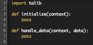
You can look at the examples of commonly-used TA-Lib functions and at our sample TA-Lib algorithm.
Daily vs minute data
The talib library respects the data frequency being passed in to it. If you pass in daily data into the library, then all the time periods are calculated in days. If you pass in minutes, then all the time periods are in minutes.
Moving average types
matype parameter. Here's the list of moving average types:0: SMA (simple) 1: EMA (exponential) 2: WMA (weighted) 3: DEMA (double exponential) 4: TEMA (triple exponential) 5: TRIMA (triangular) 6: KAMA (Kaufman adaptive) 7: MAMA (Mesa adaptive) 8: T3 (triple exponential T3)
Examples of Commonly Used Talib Functions
ATR
This algorithm uses ATR as a momentum strategy to identify price breakouts.
Clone Algorithm# This strategy was taken from http://www.investopedia.com/articles/trading/08/atr.asp
# The idea is to use ATR to identify breakouts, if the price goes higher than
# the previous close + ATR, a price breakout has occurred. The position is closed when
# the price goes 1 ATR below the previous close.
# This algorithm uses ATR as a momentum strategy, but the same signal can be used for
# a reversion strategy, since ATR doesn't indicate the price direction.
import talib
import numpy as np
import pandas as pd
# Setup our variables
def initialize(context):
# SPY
context.spy = sid(8554)
# Algorithm will only take long positions.
# It will stop if encounters a short position.
set_long_only()
schedule_function(rebalance, date_rules.every_day(), time_rules.market_open())
# Rebalance daily.
def rebalance(context, data):
# Track our position
current_position = context.portfolio.positions[context.spy].amount
record(position_size=current_position)
# Load historical data for the stocks
hist = data.history(context.spy, ['high', 'low', 'close'], 30, '1d')
# Calculate the ATR for the stock
atr = talib.ATR(hist['high'],
hist['low'],
hist['close'],
timeperiod=14)[-1]
price = data.current(context.spy, 'price')
# Use the close price from yesterday because we trade at market open
prev_close = hist['close'][-2]
# An upside breakout occurs when the price goes 1 ATR above the previous close
upside_signal = price - (prev_close + atr)
# A downside breakout occurs when the previous close is 1 ATR above the price
downside_signal = prev_close - (price + atr)
# Enter position when an upside breakout occurs. Invest our entire portfolio to go long.
if upside_signal > 0 and current_position <= 0 and data.can_trade(context.spy):
order_target_percent(context.spy, 1.0)
# Exit position if a downside breakout occurs
elif downside_signal > 0 and current_position >= 0 and data.can_trade(context.spy):
order_target_percent(context.spy, 0.0)
record(upside_signal=upside_signal,
downside_signal=downside_signal,
ATR=atr)
Bollinger Bands
This example uses the talib Bollinger Bands function to determine entry points for long and short positions. When the the price breaks out of the upper Bollinger band, a short position is opened. A long position is created when the price dips below the lower band.
Clone Algorithm# This algorithm uses the talib Bollinger Bands function to determine entry entry
# points for long and short positions.
# When the price breaks out of the upper Bollinger band, a short position
# is opened. A long position is opened when the price dips below the lower band.
import talib
import numpy as np
import pandas as pd
# Setup our variables
def initialize(context):
# SPY
context.spy = sid(8554)
schedule_function(rebalance, date_rules.every_day(), time_rules.market_open())
# Rebalance daily.
def rebalance(context, data):
current_position = context.portfolio.positions[context.spy].amount
price=data.current(context.spy, 'price')
# Load historical data for the stocks
prices = data.history(context.spy, 'price', 15, '1d')
upper, middle, lower = talib.BBANDS(
prices,
timeperiod=10,
# number of non-biased standard deviations from the mean
nbdevup=2,
nbdevdn=2,
# Moving average type: simple moving average here
matype=0)
# If price is below the recent lower band and we have
# no long positions then invest the entire
# portfolio value into SPY
if price <= lower[-1] and current_position <= 0 and data.can_trade(context.spy):
order_target_percent(context.spy, 1.0)
# If price is above the recent upper band and we have
# no short positions then invest the entire
# portfolio value to short SPY
elif price >= upper[-1] and current_position >= 0 and data.can_trade(context.spy):
order_target_percent(context.spy, -1.0)
record(upper=upper[-1],
lower=lower[-1],
mean=middle[-1],
price=price,
position_size=current_position)
MACD
In this example, when the MACD signal less than 0, the stock price is trending down and it's time to sell the security. When the MACD signal greater than 0, the stock price is trending up it's time to buy.
Clone Algorithm# This example algorithm uses the Moving Average Crossover Divergence (MACD) indicator as a buy/sell signal.
# When the MACD signal less than 0, the stock price is trending down and it's time to sell.
# When the MACD signal greater than 0, the stock price is trending up it's time to buy.
# Because this algorithm uses the history function, it will only run in minute mode.
# We will constrain the trading to once per day at market open in this example.
import talib
import numpy as np
import pandas as pd
# Setup our variables
def initialize(context):
context.stocks = symbols('MMM', 'SPY', 'GOOG_L', 'PG', 'DIA')
context.pct_per_stock = 1.0 / len(context.stocks)
schedule_function(rebalance, date_rules.every_day(), time_rules.market_open())
# Rebalance daily.
def rebalance(context, data):
# Load historical data for the stocks
prices = data.history(context.stocks, 'price', 40, '1d')
macds = {}
# Iterate over the list of stocks
for stock in context.stocks:
# Create the MACD signal and pass in the three parameters: fast period, slow period, and the signal.
macd_raw, signal, hist = talib.MACD(prices[stock], fastperiod=12,
slowperiod=26, signalperiod=9)
macd = macd_raw[-1] - signal[-1]
macds[stock] = macd
current_position = context.portfolio.positions[stock].amount
# Close position for the stock when the MACD signal is negative and we own shares.
if macd < 0 and current_position > 0 and data.can_trade(stock):
order_target(stock, 0)
# Enter the position for the stock when the MACD signal is positive and
# our portfolio shares are 0.
elif macd > 0 and current_position == 0 and data.can_trade(stock):
order_target_percent(stock, context.pct_per_stock)
record(goog=macds[symbol('GOOG_L')],
spy=macds[symbol('SPY')],
mmm=macds[symbol('MMM')])
RSI
Use the RSI signal to drive algorithm buying and selling decisions. When the RSI is over 70, a stock can be seen as overbought and it's time to sell. On the other hand, when the RSI is below 30, a stock can be seen as underbought and it's time to buy.
Clone Algorithm# This example algorithm uses the Relative Strength Index indicator as a buy/sell signal.
# When the RSI is over 70, a stock can be seen as overbought and it's time to sell.
# When the RSI is below 30, a stock can be seen as oversold and it's time to buy.
import talib
# Setup our variables
def initialize(context):
context.stocks = symbols('MMM', 'SPY', 'GE')
context.target_pct_per_stock = 1.0 / len(context.stocks)
context.LOW_RSI = 30
context.HIGH_RSI = 70
schedule_function(rebalance, date_rules.every_day(), time_rules.market_open())
# Rebalance daily.
def rebalance(context, data):
# Load historical data for the stocks
prices = data.history(context.stocks, 'price', 20, '1d')
rsis = {}
# Loop through our list of stocks
for stock in context.stocks:
# Get the rsi of this stock.
rsi = talib.RSI(prices[stock], timeperiod=14)[-1]
rsis[stock] = rsi
current_position = context.portfolio.positions[stock].amount
# RSI is above 70 and we own shares, time to sell
if rsi > context.HIGH_RSI and current_position > 0 and data.can_trade(stock):
order_target(stock, 0)
# RSI is below 30 and we don't have any shares, time to buy
elif rsi < context.LOW_RSI and current_position == 0 and data.can_trade(stock):
order_target_percent(stock, context.target_pct_per_stock)
# record the current RSI values of each stock
record(ge_rsi=rsis[symbol('GE')],
spy_rsi=rsis[symbol('SPY')],
mmm_rsi=rsis[symbol('MMM')])
STOCH
Below is an algorithm that uses the talib STOCH function. When the stochastic oscillator dips below 10, the stock is determined to be oversold and a long position is opened. The position is exited when the indicator rises above 90 because the stock is considered to be overbought.
Clone Algorithm# This algorithm uses talib's STOCH function to determine entry and exit points.
# When the stochastic oscillator dips below 10, the stock is determined to be oversold
# and a long position is opened. The position is exited when the indicator rises above 90
# because the stock is thought to be overbought.
import talib
import numpy as np
import pandas as pd
# Setup our variables
def initialize(context):
context.stocks = symbols('SPY', 'AAPL', 'GLD', 'AMZN')
# Set the percent of the account to be invested per stock
context.long_pct_per_stock = 1.0 / len(context.stocks)
schedule_function(rebalance, date_rules.every_day(), time_rules.market_open())
# Rebalance daily.
def rebalance(context, data):
# Load historical data for the stocks
hist = data.history(context.stocks, ['high', 'low', 'close'], 30, '1d')
# Iterate over our list of stocks
for stock in context.stocks:
current_position = context.portfolio.positions[stock].amount
slowk, slowd = talib.STOCH(hist['high'][stock],
hist['low'][stock],
hist['close'][stock],
fastk_period=5,
slowk_period=3,
slowk_matype=0,
slowd_period=3,
slowd_matype=0)
# get the most recent value
slowk = slowk[-1]
slowd = slowd[-1]
# If either the slowk or slowd are less than 10, the stock is
# 'oversold,' a long position is opened if there are no shares
# in the portfolio.
if slowk < 10 or slowd < 10 and current_position <= 0 and data.can_trade(stock):
order_target_percent(stock, context.long_pct_per_stock)
# If either the slowk or slowd are larger than 90, the stock is
# 'overbought' and the position is closed.
elif slowk > 90 or slowd > 90 and current_position >= 0 and data.can_trade(stock):
order_target(stock, 0)
Common Error Messages
Below are examples and sample solutions to commonly-encountered errors while coding your strategy. If you need assistance, contact us and we can help you debug the algorithm.
ExecutionTimeout
- Optimize your code to use faster functions. For example, make sure you aren't making redundant calls to history().
- Use a smaller universe of securities. Every security you include in the algorithm increases memory and CPU requirements of the algorithm.
- Backtest over a small time period.
KeyError
- Incorrect use of a dictionary. Mapping key is not found in the set of existing keys.
- Security price data is missing for the given bar, since every stock doesn't trade each minute. This often happens in the case of illiquid securities.
- Fetcher data is missing for the given bar, since Fetcher will populate your data object only when there is data for the given date.
- For missing keys in a dictionary, check that the key exists within the dictionary object. For example:
if 'blank' in dict_obj:
    value = dict_obj['blank']
LinAlgError
MemoryError
- Avoid creating too many objects or unusually large objects in your algorithm. An object can be a variable, function, or data structure.
- Use a smaller universe of securities. Every security you include in the algorithm increases memory and CPU requirements of the algorithm.
- Avoid accumulating an increasing amount of data in each bar of the backtest.
- Backtest over a shorter time period.
Something went wrong on our end. Sorry for the inconvenience.
SyntaxError
TypeError
ValueError
- Perform legal operations on expected values.
- If you run into the following error, then your code needs to specify which elements in the array are being compared.
ValueError: The truth value of a DataFrame is ambiguous. Use a.empty, a.bool(), a.item(), a.any() or a.all().. In the example below, the last elements in two lists are being compared.
if list_one[-1] > list_two[-1]:
   #ordering logic
IDE Tips and Shortcuts
You can customize the color and text size of the IDE for your algorithms. Simply click on the gear button in the top right corner and choose your settings.

Below are keyboard shortcuts you can use in the IDE.
| Action | Windows Keystroke | Apple Keystroke |
|---|---|---|
| Build Algorithm | Ctrl + B | Cmd + B |
| Indent | Ctrl + ] | Cmd + ] |
| Outdent | Ctrl + [ | Cmd + [ |
| Create/Remove Comment | Ctrl + / | Cmd + / |
| Search Code | Ctrl + F | Cmd + F |
| Undo | Ctrl + Z | Cmd + Z |
| Redo | Ctrl + Y | Cmd + Y |
Need more space to see your code? Drag the bar all the way to the right to expand the code window.

If you are building a custom graph you can record up to five variables. To view only certain variables, click on the variable name to remove it from the chart. Click it again to add it back to the graph. Want to zoom in on a certain timeperiod? Use the bar underneath the graph to select a specific time window.
Below is an example of a custom graph with all the variables selected. The following graph displays only the recorded cash value.


Research Environment API
The research environment and the IDE/backtester have different APIs. The following sections describe the functions that are available in only research. Take a look at the API Reference sample notebook to try these functions out for yourself.
Functions listed below are importable from quantopian.research:
-
quantopian.research.run_pipeline(pipeline, start_date, end_date, chunksize=None) Compute values for pipeline in number of days equal to chunksize and return stitched up result. Computing in chunks is useful for pipelines computed over a long period of time.
Parameters: Returns: result (pd.DataFrame) – A frame of computed results.
The
resultcolumns correspond to the entries of pipeline.columns, which should be a dictionary mapping strings to instances ofzipline.pipeline.term.Term.For each date between
start_dateandend_date,resultwill contain a row for each asset that passed pipeline.screen. A screen ofNoneindicates that a row should be returned for each asset that existed each day.
-
quantopian.research.symbols(symbols, symbol_reference_date=None, handle_missing='log') Convert a string or a list of strings into Asset objects.
Parameters: - symbols (String or iterable of strings.) – Passed strings are interpreted as ticker symbols and resolved relative to the date specified by symbol_reference_date.
- symbol_reference_date (str or pd.Timestamp, optional) – String or Timestamp representing a date used to resolve symbols that have been held by multiple companies. Defaults to the current time.
- handle_missing ({'raise', 'log', 'ignore'}, optional) – String specifying how to handle unmatched securities. Defaults to ‘log’.
Returns: list of Asset objects – The symbols that were requested.
-
quantopian.research.prices(assets, start, end, frequency='daily', price_field='price', symbol_reference_date=None, start_offset=0) Get close price data for assets between start and end.
Parameters: - assets (int/str/Asset or iterable of same) – Identifiers for assets to load. Integers are interpreted as sids. Strings are interpreted as symbols.
- start (str or pd.Timestamp) – Start date of data to load.
- end (str or pd.Timestamp) – End date of data to load.
- frequency ({'minute', 'daily'}, optional) – Frequency at which to load data. Default is ‘daily’.
- price_field ({'open', 'high', 'low', 'close', 'price'}, optional) – Price field to load. ‘price’ produces the same data as ‘close’, but forward-fills over missing data. Default is ‘price’.
- symbol_reference_date (pd.Timestamp, optional) – Date as of which to resolve strings as tickers. Default is the current day.
- start_offset (int, optional) – Number of periods before
startto fetch. Default is 0. This is most often useful for calculating returns.
Returns: prices (pd.Series or pd.DataFrame) – Pandas object containing prices for the requested asset(s) and dates.
Data is returned as a
pd.Seriesif a single asset is passed.Data is returned as a
pd.DataFrameif multiple assets are passed.
-
quantopian.research.returns(assets, start, end, periods=1, frequency='daily', price_field='price', symbol_reference_date=None) Fetch returns for one or more assets in a date range.
Parameters: - assets (int/str/Asset or iterable of same) – Identifiers for assets to load. Integers are interpreted as sids. Strings are interpreted as symbols.
- start (str or pd.Timestamp) – Start date of data to load.
- end (str or pd.Timestamp) – End date of data to load.
- periods (int, optional) – Number of periods over which to calculate returns. Default is 1.
- frequency ({'minute', 'daily'}, optional) – Frequency at which to load data. Default is ‘daily’.
- price_field ({'open', 'high', 'low', 'close', 'price'}, optional) – Price field to load. ‘price’ produces the same data as ‘close’, but forward-fills over missing data. Default is ‘price’.
- symbol_reference_date (pd.Timestamp, optional) – Date as of which to resolve strings as tickers. Default is the current day.
Returns: returns (pd.Series or pd.DataFrame) – Pandas object containing returns for the requested asset(s) and dates.
Data is returned as a
pd.Seriesif a single asset is passed.Data is returned as a
pd.DataFrameif multiple assets are passed.
-
quantopian.research.volumes(assets, start, end, frequency='daily', symbol_reference_date=None, start_offset=0) Get trading volume for assets between start and end.
Parameters: - assets (int/str/Asset or iterable of same) – Identifiers for assets to load. Integers are interpreted as sids. Strings are interpreted as symbols.
- start (str or pd.Timestamp) – Start date of data to load.
- end (str or pd.Timestamp) – End date of data to load.
- frequency ({'minute', 'daily'}, optional) – Frequency at which to load data. Default is ‘daily’.
- symbol_reference_date (pd.Timestamp, optional) – Date as of which to resolve strings as tickers. Default is the current day.
- start_offset (int, optional) – Number of periods before
startto fetch. Default is 0. This is most often useful for calculating returns.
Returns: volumes (pd.Series or pd.DataFrame) – Pandas object containing volumes for the requested asset(s) and dates.
Data is returned as a
pd.Seriesif a single asset is passed.Data is returned as a
pd.DataFrameif multiple assets are passed.
-
quantopian.research.log_prices(assets, start, end, frequency='daily', price_field='price', symbol_reference_date=None, start_offset=0) Fetch logarithmic-prices for one or more assets in a date range.
Parameters: - assets (int/str/Asset or iterable of same) – Identifiers for assets to load. Integers are interpreted as sids. Strings are interpreted as symbols.
- start (str or pd.Timestamp) – Start date of data to load.
- end (str or pd.Timestamp) – End date of data to load.
- frequency ({'minute', 'daily'}, optional) – Frequency at which to load data. Default is ‘daily’.
- price_field ({'open', 'high', 'low', 'close', 'price'}, optional) – Price field to load. ‘price’ produces the same data as ‘close’, but forward-fills over missing data. Default is ‘price’.
- symbol_reference_date (pd.Timestamp, optional) – Date as of which to resolve strings as tickers. Default is the current day.
- start_offset (int, optional) – Number of periods before
startto fetch. Default is 0. This is most often useful for calculating returns.
Returns: prices (pd.Series or pd.DataFrame) – Pandas object containing log-prices for the requested asset(s) and dates.
Data is returned as a
pd.Seriesif a single asset is passed.Data is returned as a
pd.DataFrameif multiple assets are passed.
-
quantopian.research.log_returns(assets, start, end, periods=1, frequency='daily', price_field='price', symbol_reference_date=None) Fetch logarithmic-returns for one or more assets in a date range.
Parameters: - assets (int/str/Asset or iterable of same) – Identifiers for assets to load. Integers are interpreted as sids. Strings are interpreted as symbols.
- start (str or pd.Timestamp) – Start date of data to load.
- end (str or pd.Timestamp) – End date of data to load.
- periods (int, optional) – Number of periods over which to calculate returns. Default is 1.
- frequency ({'minute', 'daily'}, optional) – Frequency at which to load data. Default is ‘daily’.
- price_field ({'open', 'high', 'low', 'close', 'price'}, optional) – Price field to load. ‘price’ produces the same data as ‘close’, but forward-fills over missing data. Default is ‘price’.
- symbol_reference_date (pd.Timestamp, optional) – Date as of which to resolve strings as tickers. Default is the current day.
Returns: returns (pd.Series or pd.DataFrame) – Pandas object containing logarithmic-returns for the requested asset(s) and dates.
Data is returned as a
pd.Seriesif a single asset is passed.Data is returned as a
pd.DataFrameif multiple assets are passed.
-
quantopian.research.get_pricing(symbols, start_date='2013-01-03', end_date='2014-01-03', symbol_reference_date=None, frequency='daily', fields=None, handle_missing='raise', start_offset=0) Load a table of historical trade data.
Parameters: - symbols (Object (or iterable of objects) convertible to Asset) – Valid input types are Asset, Integral, or basestring. In the case that the passed objects are strings, they are interpreted as ticker symbols and resolved relative to the date specified by symbol_reference_date.
- start_date (str or pd.Timestamp, optional) – String or Timestamp representing a start date or start intraday minute for the returned data. Defaults to ‘2013-01-03’.
- end_date (str or pd.Timestamp, optional) – String or Timestamp representing an end date or end intraday minute for the returned data. Defaults to ‘2014-01-03’.
- symbol_reference_date (str or pd.Timestamp, optional) – String or Timestamp representing a date used to resolve symbols that have been held by multiple companies. Defaults to the current time.
- frequency ({'daily', 'minute'}, optional) – Resolution of the data to be returned.
- fields (str or list, optional) – String or list drawn from {‘price’, ‘open_price’, ‘high’, ‘low’, ‘close_price’, ‘volume’}. Default behavior is to return all fields.
- handle_missing ({'raise', 'log', 'ignore'}, optional) – String specifying how to handle unmatched securities. Defaults to ‘raise’.
- start_offset (int, optional) – Number of periods before
startto fetch. Default is 0.
Returns: pandas Panel/DataFrame/Series – The pricing data that was requested. See note below.
Notes
If a list of symbols is provided, data is returned in the form of a pandas Panel object with the following indices:
items = fields
major_axis = TimeSeries (start_date -> end_date)
minor_axis = symbols
If a string is passed for the value of symbols and fields is None or a list of strings, data is returned as a DataFrame with a DatetimeIndex and columns given by the passed fields.
If a list of symbols is provided, and fields is a string, data is returned as a DataFrame with a DatetimeIndex and a columns given by the passed symbols.
If both parameters are passed as strings, data is returned as a Series.
-
quantopian.research.get_backtest(backtest_id) Get the results of a backtest that was run on Quantopian.
Parameters: backtest_id (str) – The id of the backtest for which results should be returned. Returns: result (AlgorithmResult) – An object containing all the information stored by Quantopian about the performance of a given backtest run, as well as some additional metadata. Notes
You can find the ID of a backtest in the URL of its full results page, which will be of the form:
https://www.quantopian.com/algorithms/<algorithm_id>/<backtest_id>
Once you have your BacktestResult object, you can call
create_full_tear_sheet()on it to get an in-depth analysis of your backtest:bt = get_backtest('<backtest_id>') bt.create_full_tear_sheet()
See also
-
quantopian.research.get_live_results(live_algo_id) Get the results of a live algorithm running on Quantopian.
Parameters: live_algo_id (str) – The id of the algorithm for which results should be returned. Returns: result (AlgorithmResult) – An object containing all the information stored by Quantopian about the performance of a given live algorithm, as well as some additional metadata. Notes
You can find the ID of a live algorithm in the URL of its full results page, which will be of the form:
https://www.quantopian.com/live_algorithms/<algorithm_id>
Once you have your LiveAlgorithmResult object, you can call
create_full_tear_sheet()on it to get an in-depth analysis of your live algorithm:lr = get_live_results('<algorithm_id>') lr.create_full_tear_sheet()
See also
-
class
quantopian.research.AlgorithmResult Container for data about the performance of an algorithm.
AlgorithmResults are returned by the following API functions:
quantopian.research.get_backtest()loads an AlgorithmResult for a completed backtest.quantopian.research.get_live_results()loads an AlgorithmResult for a live algorithm.
-
create_full_tear_sheet(benchmark_rets=None, slippage=None, live_start_date=None, bayesian=False, round_trips=False, estimate_intraday='infer', hide_positions=False, cone_std=(1.0, 1.5, 2.0), bootstrap=False, header_rows=None) Generate a number of tear sheets that are useful for analyzing a strategy’s performance.
Creates tear sheets for returns, significant events, positions, transactions, and Bayesian analysis.
Parameters: - benchmark_rets (pd.Series or pd.DataFrame, optional) – Daily noncumulative returns of the benchmark. This is in the same style as returns.
- slippage (int/float, optional) – Basis points of slippage to apply to returns before generating tearsheet stats and plots. If a value is provided, slippage parameter sweep plots will be generated from the unadjusted returns. See pyfolio.txn.adjust_returns_for_slippage for more details.
- live_start_date (datetime, optional) – The point in time when the strategy began live trading, after its backtest period.
- bayesian (boolean, optional) – If True, causes the generation of a Bayesian tear sheet.
- round_trips (boolean, optional) – If True, causes the generation of a round trip tear sheet.
- estimate_intraday (boolean or str, optional) – Instead of using the end-of-day positions, use the point in the day where we have the most $ invested. This will adjust positions to better approximate and represent how an intraday strategy behaves. By default, this is ‘infer’, and an attempt will be made to detect an intraday strategy. Specifying this value will prevent detection.
- hide_positions (bool, optional) – If True, will not output any symbol names.
- cone_std (float, or tuple, optional) – If float, the standard deviation to use for the cone plots. If tuple, tuple of stdev values to use for the cone plots. The cone is a normal distribution with this standard deviation centered around a linear regression.
- bootstrap (boolean, optional) – Whether to perform bootstrap analysis for the performance metrics. Takes a few minutes longer.
- header_rows (dict or OrderedDict, optional) – Extra rows to display at the top of the perf stats table.
-
create_perf_attrib_tear_sheet(return_fig=False) Generate plots and tables for analyzing a strategy’s performance.
Parameters: return_fig (boolean, optional) – If True, returns the figure that was plotted on.
-
create_simple_tear_sheet(benchmark_rets=None, slippage=None, live_start_date=None, estimate_intraday='infer', header_rows=None) Simpler version of create_full_tear_sheet; generates summary performance statistics and important plots as a single image.
Parameters: - benchmark_rets (pd.Series or pd.DataFrame, optional) – Daily noncumulative returns of the benchmark. This is in the same style as returns.
- slippage (int/float, optional) – Basis points of slippage to apply to returns before generating tearsheet stats and plots. If a value is provided, slippage parameter sweep plots will be generated from the unadjusted returns. See pyfolio.txn.adjust_returns_for_slippage for more details.
- live_start_date (datetime, optional) – The point in time when the strategy began live trading, after its backtest period.
- estimate_intraday (boolean or str, optional) – Instead of using the end-of-day positions, use the point in the day where we have the most $ invested. This will adjust positions to better approximate and represent how an intraday strategy behaves. By default, this is ‘infer’, and an attempt will be made to detect an intraday strategy. Specifying this value will prevent detection.
- header_rows (dict or OrderedDict, optional) – Extra rows to display at the top of the perf stats table.
-
preview(attr, length=3, transpose=True) Return a preview of the first length bars of the timeseries stored in getattr(self, attr).
If transpose == True (the default), then the result is transposed before being returned.
-
algo_id Return the algorithm’s ID
-
attributed_factor_returns Return a daily datetime-indexed DataFrame containing the algorithm’s returns broken down by style and sector risk factors. Also includes columns for common returns (sum of returns from known factors), specific returns (alpha), and total returns.
Each row of the returned frame contains the following columns:
- basic_materials
- consumer_cyclical
- financial_services
- real_estate
- consumer_defensive
- health_care
- utilities
- communication_services
- energy
- industrials
- technology
- momentum
- size
- value
- short_term_reversal
- volatility
- common_returns
- specific_returns
- total_returns
Example output:
            basic_materials  ...  volatility  common_returns  specific_returns    total_returns
dt
2017-01-09   0.000000             -0.000091   -0.000127        0.000437           -0.000869
2017-01-10   0.000034              0.000422    0.000076        0.000663            0.000426
2017-01-11   0.000373              0.000192    0.000089        0.000261            0.000689
2017-01-12  -0.000093             -0.000039   -0.000139       -0.000244           -0.000462
2017-01-13  -0.000085              0.000284    0.000095        0.000059            0.000689
-
benchmark_security Return the security used as a benchmark for this algorithm.
-
capital_base Return the capital base for this algorithm.
-
cumulative_performance Return a DataFrame with a daily DatetimeIndex containing cumulative performance metrics for the algorithm.
Each row of the returned frame contains the following columns:
- capital_used
- starting_cash
- ending_cash
- starting_position_value
- ending_position_value
- pnl
- portfolio_value
- returns
-
daily_performance Return a DataFrame with a daily DatetimeIndex containing cumulative performance metrics for the algorithm
Each row of the returned frame contains the following columns:
- capital_used
- starting_cash
- ending_cash
- starting_position_value
- ending_position_value
- pnl
- portfolio_value
- returns
-
end_date Return the end date for this algorithm.
-
factor_exposures Return a daily datetime-indexed DataFrame containing the algorithm’s exposures to style and sector risk factors.
Factor exposures are calculated by taking the algorithm’s (dates x assets) matrix of portfolio weights each day and multiplying by the (assets x factors) loadings matrix produced by the Quantopian Risk Model. The result is a (dates x factors) matrix representing the factor-weighted sum of the algorithms holdings for each factor on each day.
Each row of the returned frame contains the following columns:
- basic_materials
- consumer_cyclical
- financial_services
- real_estate
- consumer_defensive
- health_care
- utilities
- communication_services
- energy
- industrials
- technology
- momentum
- size
- value
- short_term_reversal
- volatility
Example output:
             basic_materials  consumer_cyclical  ...  technology  momentum  ...  volatility
dt
2017-01-09   0.0              0.0                     0.788057    0.175617       -0.208708
2017-01-10   0.0              0.0                     1.180821    0.274301       -0.314133
2017-01-11   0.0              0.0                     0.654444    0.190959       -0.173934
2017-01-12   0.0              0.0                     0.768404    0.181316       -0.207495
2017-01-13   0.0              0.0                     1.522823    0.325506       -0.382107
-
launch_date The real-world date on which this algorithm launched.
-
orders Return a DataFrame representing a record of all orders made by the algorithm.
Each row of the returned frame contains the following columns:
- amount
- commission
- created_date
- last_updated
- filled
- id
- sid
- status
- limit
- limit_reached
- stop
- stop_reached
-
positions Return a datetime-indexed DataFrame representing a point-in-time record of positions held by the algorithm during the backtest.
Each row of the returned frame contains the following columns:
- amount
- last_sale_price
- cost_basis
- sid
-
pyfolio_positions Return a DataFrame containing positions formatted for pyfolio.
-
pyfolio_transactions Return a DataFrame containing transactions formatted for pyfolio.
-
recorded_vars Return a DataFrame containing the recorded variables for the algorithm.
-
risk Return a DataFrame with a daily DatetimeIndex representing rolling risk metrics for the algorithm.
Each row of the returned frame contains the following columns:
- volatility
- period_return
- alpha
- benchmark_period_return
- benchmark_volatility
- beta
- excess_return
- max_drawdown
- period_label
- sharpe
- sortino
- trading_days
- treasury_period_return
-
start_date Return the start date for this algorithm.
-
transactions Return a DataFrame representing a record of transactions that occurred during the life of the algorithm. The returned frame is indexed by the date at which the transaction occurred.
Each row of the returned frame contains the following columns:
- amount
- commission
- date
- order_id
- price
- sid
-
quantopian.research.local_csv(path, symbol_column=None, date_column=None, use_date_column_as_index=True, timezone='UTC', symbol_reference_date=None, **read_csv_kwargs) Load a CSV from the /data directory.
Parameters: - path (str) – Path of file to load, relative to /data.
- symbol_column (string, optional) – Column containing strings to convert to Asset objects.
- date_column (str, optional) – Column to parse as Datetime. Ignored if parse_dates is passed as an additional keyword argument.
- use_date_column_as_index (bool, optional) – If True and date_column is supplied, set it as the frame index.
- timezone (str or pytz.timezone object, optional) – Interpret date_column as this timezone.
- symbol_reference_date (str or pd.Timestamp, optional) – String or Timestamp representing a date used to resolve symbols that have been held by multiple companies. Defaults to the current time.
- read_csv_kwargs (optional) – Extra parameters to forward to pandas.read_csv.
Returns: pandas.DataFrame – DataFrame with data from the loaded file.
Experimental Research API
The following functions have been recently added to the Research API. They are
importable from quantopian.research.experimental.
We expect to eventually stabilize these APIs and move the functions into the
core quantopian.research: module.
-
quantopian.research.experimental.get_factor_loadings(assets, start, end, handle_missing='log') Retrieve Quantopian Risk Model loadings for a given period.
Parameters: - assets (int/str/Asset or iterable of same) – Identifiers for assets to load. Integers are interpreted as sids. Strings are interpreted as symbols.
- start (str or pd.Timestamp) – Start date of data to load.
- end (str or pd.Timestamp) – End date of data to load.
- handle_missing ({'raise', 'log', 'ignore'}, optional) – String specifying how to handle unmatched securities. Defaults to ‘log’.
-
quantopian.research.experimental.get_factor_returns(start, end) Retrieve Quantopian Risk Model factor returns for a given period.
Parameters: - start (str or pd.Timestamp) – Start date of data to load.
- end (str or pd.Timestamp) – End date of data to load.
Returns: factor_returns (
pandas.DataFrame) – ADataFramecontaining returns for each factor calculated by the Quantopian Risk Model.
-
quantopian.research.experimental.continuous_future(root_symbol, offset=0, roll='volume', adjustment='mul') Create a specifier for a continuous contract.
Parameters: - root_symbol (str) – The root symbol for the continuous future.
- offset (int, optional) – The distance from the primary contract. Default is 0.
- roll (str, optional) – How rolls are determined. Options are ‘volume’ and ‘calendar’. Default is ‘volume’.
- adjustment (str) – Method for adjusting lookback prices between rolls. Options are ‘mul’, ‘add’, and None. Default is ‘mul’.
Returns: continuous_future (ContinuousFuture) – The continuous future specifier.
-
quantopian.research.experimental.history(symbols, fields, start, end, frequency, symbol_reference_date=None, handle_missing='raise', start_offset=0) Load a table of historical trade data.
Parameters: - symbols (Asset-convertible object, ContinuousFuture, or iterable of same.) – Valid input types are Asset, Integral, basestring, or ContinuousFuture. In the case that the passed objects are strings, they are interpreted as ticker symbols and resolved relative to the date specified by symbol_reference_date.
- fields (str or list) – String or list drawn from {‘price’, ‘open_price’, ‘high’, ‘low’, ‘close_price’, ‘volume’, ‘contract’}.
- start (str or pd.Timestamp) – String or Timestamp representing a start date or start intraday minute for the returned data.
- end (str or pd.Timestamp) – String or Timestamp representing an end date or end intraday minute for the returned data.
- frequency ({'daily', 'minute'}) – Resolution of the data to be returned.
- symbol_reference_date (str or pd.Timestamp, optional) – String or Timestamp representing a date used to resolve symbols that have been held by multiple companies. Defaults to the current time.
- handle_missing ({'raise', 'log', 'ignore'}, optional) – String specifying how to handle unmatched securities. Defaults to ‘raise’.
- start_offset (int, optional) – Number of periods before
startto fetch. Default is 0. This is most often useful when computing returns.
Returns: pandas Panel/DataFrame/Series – The pricing data that was requested. See note below.
Notes
If a list of symbols is provided, data is returned in the form of a pandas Panel object with the following indices:
items = fields
major_axis = TimeSeries (start_date -> end_date)
minor_axis = symbols
If a string is passed for the value of symbols and fields is None or a list of strings, data is returned as a DataFrame with a DatetimeIndex and columns given by the passed fields.
If a list of symbols is provided, and fields is a string, data is returned as a DataFrame with a DatetimeIndex and a columns given by the passed symbols.
If both parameters are passed as strings, data is returned as a Series.
Sample Algorithms
Below are examples to help you learn the Quantopian functions and backtest in the IDE. Clone an algorithm to get your own copy.
The material on this website is provided for informational purposes only and does not constitute an offer to sell, a solicitation to buy, or a recommendation or endorsement for any security or strategy, nor does it constitute an offer to provide investment advisory services by Quantopian.
In addition, the material offers no opinion with respect to the suitability of any security or specific investment. No information contained herein should be regarded as a suggestion to engage in or refrain from any investment-related course of action as none of Quantopian nor any of its affiliates is undertaking to provide investment advice, act as an adviser to any plan or entity subject to the Employee Retirement Income Security Act of 1974, as amended, individual retirement account or individual retirement annuity, or give advice in a fiduciary capacity with respect to the materials presented herein. If you are an individual retirement or other investor, contact your financial advisor or other fiduciary unrelated to Quantopian about whether any given investment idea, strategy, product or service described herein may be appropriate for your circumstances. All investments involve risk, including loss of principal. Quantopian makes no guarantees as to the accuracy or completeness of the views expressed in the website. The views are subject to change, and may have become unreliable for various reasons, including changes in market conditions or economic circumstances.
Basic Algorithm
This example demonstrates all of the basic concepts you need to write a simple algorithm that tries to capitalize on a stock's momentum. This shows you the symbol function, logging, volume-weighted average price, price, and placing orders. You clone this algorithm below or from the community discussion of this post.
Clone Algorithm"""
For this example, we're going to write a simple momentum script.
When the stock goes up quickly, we're going to buy;
when it goes down we're going to sell.
Hopefully we'll ride the waves.
To run an algorithm in Quantopian, you need to define two functions:
initialize and handle_data.
Note: AAPL had a 7:1 split in June 2014, which is reflected in the
recorded variables plot.
"""
"""
The initialize function sets any data or variables that
you'll use in your algorithm.
It's only called once at the beginning of your algorithm.
"""
def initialize(context):
# In our example, we're looking at Apple. If you re-type
# this line you'll see the auto-complete popup after `sid(`.
context.security = sid(24)
# Specify that we want the 'rebalance' method to run once a day
schedule_function(rebalance, date_rule=date_rules.every_day())
"""
Rebalance function scheduled to run once per day (at market open).
"""
def rebalance(context, data):
# To make market decisions, we're calculating the stock's
# moving average for the last 5 days.
# We get the price history for the last 5 days.
price_history = data.history(
context.security,
fields='price',
bar_count=5,
frequency='1d'
)
# Then we take an average of those 5 days.
average_price = price_history.mean()
# We also get the stock's current price.
current_price = data.current(context.security, 'price')
# If our stock is currently listed on a major exchange
if data.can_trade(context.security):
# If the current price is 1% above the 5-day average price,
# we open a long position. If the current price is below the
# average price, then we want to close our position to 0 shares.
if current_price > (1.01 * average_price):
# Place the buy order (positive means buy, negative means sell)
order_target_percent(context.security, 1)
log.info("Buying %s" % (context.security.symbol))
elif current_price < average_price:
# Sell all of our shares by setting the target position to zero
order_target_percent(context.security, 0)
log.info("Selling %s" % (context.security.symbol))
# Use the record() method to track up to five custom signals.
# Record Apple's current price and the average price over the last
# five days.
record(current_price=current_price, average_price=average_price)
Schedule Function
This example uses schedule_function() to rebalance at 11:00AM once per week on the first trading day of that week. Clone the algorithm to get your own copy where you can change the securitites and rebalancing window.
"""
This algorithm defines a long-only equal weight portfolio and
rebalances it at a user-specified frequency.
"""

# Import the libraries we will use here
import datetime
import pandas as pd

def initialize(context):
    # In this example, we're looking at 9 sector ETFs.
    context.security_list = symbols('XLY',  # XLY Consumer Discretionary SPDR Fund
                           'XLF',  # XLF Financial SPDR Fund
                           'XLK',  # XLK Technology SPDR Fund
                           'XLE',  # XLE Energy SPDR Fund
                           'XLV',  # XLV Health Care SPRD Fund
                           'XLI',  # XLI Industrial SPDR Fund
                           'XLP',  # XLP Consumer Staples SPDR Fund
                           'XLB',  # XLB Materials SPDR Fund
                           'XLU')  # XLU Utilities SPRD Fund

    # This variable is used to manage leverage
    context.weights = 0.99/len(context.security_list)

    # Rebalance every day (or the first trading day if it's a holiday).
    # At 11AM ET, which is 1 hour and 30 minutes after market open.
    schedule_function(rebalance,
                      date_rules.week_start(days_offset=0),
                      time_rules.market_open(hours = 1, minutes = 30))

def rebalance(context, data):

    # Do the rebalance. Loop through each of the stocks and order to
    # the target percentage.  If already at the target, this command
    # doesn't do anything. A future improvement could be to set rebalance
    # thresholds.
    for sec in context.security_list:
        if data.can_trade(sec):
            order_target_percent(sec, context.weights)

    # Get the current exchange time, in the exchange timezone
    exchange_time = get_datetime('US/Eastern')
    log.info("Rebalanced to target portfolio weights at %s" % str(exchange_time))
Pipeline
Pipeline Basics
In this algo, you will learn about creating and attaching a pipeline, adding factors and filters, setting screens, and accessing the output of your pipeline.
Clone Algorithm# The pipeline API requires imports.
from quantopian.pipeline import Pipeline
from quantopian.algorithm import attach_pipeline, pipeline_output
from quantopian.pipeline.data.builtin import USEquityPricing
from quantopian.pipeline.factors import SimpleMovingAverage, AverageDollarVolume
def initialize(context):
# Construct a simple moving average factor
sma = SimpleMovingAverage(inputs=[USEquityPricing.close], window_length=10)
# Construct a 30-day average dollar volume factor
dollar_volume = AverageDollarVolume(window_length=30)
# Define high dollar-volume filter to be the top 2% of stocks by dollar volume.
high_dollar_volume = dollar_volume.percentile_between(98, 100)
# Set a screen on the pipelines to filter out securities.
pipe_screen = ((sma > 1.0) & high_dollar_volume)
# Create a columns dictionary
pipe_columns = {'dollar_volume':dollar_volume, 'sma':sma}
# Create, register and name a pipeline in initialize.
pipe = Pipeline(columns=pipe_columns,screen=pipe_screen)
attach_pipeline(pipe, 'example')
def before_trading_start(context, data):
# Pipeline_output returns the constructed dataframe.
output = pipeline_output('example')
# Select and update your universe.
context.my_securities = output.sort('sma', ascending=False).iloc[:50]
print len(context.my_securities)
context.security_list = context.my_securities.index
log.info("\n" + str(context.my_securities.head(5)))
Combining and Ranking
This example shows that factors can be combined to create new factors, that factors can be ranked using masks, and how you can use the pipeline API to create long and short lists.
Clone Algorithmfrom quantopian.algorithm import attach_pipeline, pipeline_output
from quantopian.pipeline import Pipeline
from quantopian.pipeline.data.builtin import USEquityPricing
from quantopian.pipeline.factors import SimpleMovingAverage
def initialize(context):
sma_short = SimpleMovingAverage(inputs=[USEquityPricing.close], window_length=30)
sma_long = SimpleMovingAverage(inputs=[USEquityPricing.close], window_length=100)
# Combined factors to create new factors
sma_quotient = sma_short / sma_long
# Create a screen to remove penny stocks
remove_penny_stocks = sma_short > 1.0
sma_rank = sma_quotient.rank(mask=remove_penny_stocks)
# Rank a factor using a mask to ignore the values we're
# filtering out by passing mask=remove_penny_stocks to rank.
longs = sma_rank.top(200, mask=remove_penny_stocks)
shorts = sma_rank.bottom(200, mask=remove_penny_stocks)
pipe_columns = {
'longs':longs,
'shorts':shorts,
'sma_rank':sma_rank
}
# Use multiple screens to narrow the universe
pipe_screen = (longs | shorts)
pipe = Pipeline(columns = pipe_columns,screen = pipe_screen)
attach_pipeline(pipe, 'example')
def before_trading_start(context, data):
context.output = pipeline_output('example')
context.longs = context.output[context.output.longs]
context.shorts = context.output[context.output.shorts]
context.security_list = context.shorts.index.union(context.longs.index)
# Print the 5 securities with the lowest sma_rank.
print "SHORT LIST"
log.info("\n" + str(context.shorts.sort(['sma_rank'], ascending=True).head()))
# Print the 5 securities with the highest sma_rank.
print "LONG LIST"
log.info("\n" + str(context.longs.sort(['sma_rank'], ascending=False).head()))
Creating Custom Factors
This example shows how custom factors can be defined and used. It also shows how pricing data and Morningstar fundamentals data can be used together.
Clone Algorithmimport quantopian.algorithm as algo
from quantopian.pipeline import CustomFactor, Pipeline
from quantopian.pipeline.data import Fundamentals
from quantopian.pipeline.data.builtin import USEquityPricing
from quantopian.pipeline.factors import AverageDollarVolume, SimpleMovingAverage
# Create custom factor subclass to calculate a market cap based on yesterday's
# close
class MarketCap(CustomFactor):
# Pre-declare inputs and window_length
inputs = [USEquityPricing.close, Fundamentals.shares_outstanding]
window_length = 1
# Compute market cap value
def compute(self, today, assets, out, close, shares):
out[:] = close[-1] * shares[-1]
def initialize(context):
# Note that we don't call add_factor on these Factors.
# We don't need to store intermediate values if we're not going to use them
sma_short = SimpleMovingAverage(inputs=[USEquityPricing.close], window_length=30)
sma_long = SimpleMovingAverage(inputs=[USEquityPricing.close], window_length=100)
sma_quotient = sma_short / sma_long
# Construct the custom factor
mkt_cap = MarketCap()
# Create and apply a filter representing the top 500 equities by MarketCap
# every day.
mkt_cap_top_500 = mkt_cap.top(500)
# Construct an average dollar volume factor
dollar_volume = AverageDollarVolume(window_length=30)
# Define high dollar-volume filter to be the top 10% of stocks by dollar
# volume.
high_dollar_volume = dollar_volume.percentile_between(90, 100)
high_cap_high_dv = mkt_cap_top_500 & high_dollar_volume
# Create filters for our long and short portfolios.
longs = sma_quotient.top(200, mask=high_cap_high_dv)
shorts = sma_quotient.bottom(200, mask=high_cap_high_dv)
pipe_columns = {
'longs': longs,
'shorts': shorts,
'mkt_cap': mkt_cap,
'sma_quotient': sma_quotient,
}
# Use multiple screens to narrow the universe
pipe_screen = (longs | shorts)
pipe = Pipeline(columns=pipe_columns, screen=pipe_screen)
algo.attach_pipeline(pipe, 'example')
def before_trading_start(context, data):
context.output = algo.pipeline_output('example')
context.longs = context.output[context.output.longs]
context.shorts = context.output[context.output.shorts]
context.security_list = context.shorts.index.union(context.longs.index)
# Print the 5 securities with the lowest sma_quotient.
print "SHORT LIST"
log.info("\n" + str(context.shorts.sort(['sma_quotient'], ascending=True).head()))
# Print the 5 securities with the highest sma_quotient.
print "LONG LIST"
log.info("\n" + str(context.longs.sort(['sma_quotient'], ascending=False).head()))
Earnings Announcement Risk Framework
This example demonstrates how to detect and react to earnings announcements in your algorithm. It uses the built-in earnings announcement pipeline data factors to avoid securities 3 days around an earnings announcement
Clone Algorithmimport numpy as np
from quantopian.algorithm import attach_pipeline, pipeline_output
from quantopian.pipeline import Pipeline
from quantopian.pipeline.data.builtin import USEquityPricing
from quantopian.pipeline.classifiers.morningstar import Sector
from quantopian.pipeline.factors import CustomFactor, AverageDollarVolume
from quantopian.pipeline.data import morningstar as mstar
from quantopian.pipeline.filters.morningstar import IsPrimaryShare
from quantopian.pipeline.data.zacks import EarningsSurprises
# The sample and full version is found through the same namespace
# https://www.quantopian.com/data/eventvestor/earnings_calendar
# Sample date ranges: 01 Jan 2007 - 10 Feb 2014
from quantopian.pipeline.data.eventvestor import EarningsCalendar
from quantopian.pipeline.factors.eventvestor import (
BusinessDaysUntilNextEarnings,
BusinessDaysSincePreviousEarnings
)
# from quantopian.pipeline.data.accern import alphaone_free as alphaone
# Premium version availabe at
# https://www.quantopian.com/data/accern/alphaone
from quantopian.pipeline.data.accern import alphaone_free as alphaone
def make_pipeline(context):
# Create our pipeline
pipe = Pipeline()
# Instantiating our factors
factor = EarningsSurprises.eps_pct_diff_surp.latest
# Filter down to stocks in the top/bottom according to
# the earnings surprise
longs = (factor >= context.min_surprise) & (factor <= context.max_surprise)
shorts = (factor <= -context.min_surprise) & (factor >= -context.max_surprise)
# Set our pipeline screens
# Filter down stocks using sentiment
article_sentiment = alphaone.article_sentiment.latest
top_universe = universe_filters() & longs & article_sentiment.notnan() \
& (article_sentiment > .30)
bottom_universe = universe_filters() & shorts & article_sentiment.notnan() \
& (article_sentiment < -.50)
# Add long/shorts to the pipeline
pipe.add(top_universe, "longs")
pipe.add(bottom_universe, "shorts")
pipe.add(BusinessDaysSincePreviousEarnings(), 'pe')
pipe.set_screen(factor.notnan())
return pipe
def initialize(context):
#: Set commissions and slippage to 0 to determine pure alpha
set_commission(commission.PerShare(cost=0, min_trade_cost=0))
set_slippage(slippage.FixedSlippage(spread=0))
#: Declaring the days to hold, change this to what you want
context.days_to_hold = 3
#: Declares which stocks we currently held and how many days we've held them dict[stock:days_held]
context.stocks_held = {}
#: Declares the minimum magnitude of percent surprise
context.min_surprise = .00
context.max_surprise = .05
#: OPTIONAL - Initialize our Hedge
# See order_positions for hedging logic
# context.spy = sid(8554)
# Make our pipeline
attach_pipeline(make_pipeline(context), 'earnings')
# Log our positions at 10:00AM
schedule_function(func=log_positions,
date_rule=date_rules.every_day(),
time_rule=time_rules.market_close(minutes=30))
# Order our positions
schedule_function(func=order_positions,
date_rule=date_rules.every_day(),
time_rule=time_rules.market_open())
def before_trading_start(context, data):
# Screen for securities that only have an earnings release
# 1 business day previous and separate out the earnings surprises into
# positive and negative
results = pipeline_output('earnings')
results = results[results['pe'] == 1]
assets_in_universe = results.index
context.positive_surprise = assets_in_universe[results.longs]
context.negative_surprise = assets_in_universe[results.shorts]
def log_positions(context, data):
#: Get all positions
if len(context.portfolio.positions) > 0:
all_positions = "Current positions for %s : " % (str(get_datetime()))
for pos in context.portfolio.positions:
if context.portfolio.positions[pos].amount != 0:
all_positions += "%s at %s shares, " % (pos.symbol, context.portfolio.positions[pos].amount)
log.info(all_positions)
def order_positions(context, data):
"""
Main ordering conditions to always order an equal percentage in each position
so it does a rolling rebalance by looking at the stocks to order today and the stocks
we currently hold in our portfolio.
"""
port = context.portfolio.positions
record(leverage=context.account.leverage)
# Check our positions for loss or profit and exit if necessary
check_positions_for_loss_or_profit(context, data)
# Check if we've exited our positions and if we haven't, exit the remaining securities
# that we have left
for security in port:
if data.can_trade(security):
if context.stocks_held.get(security) is not None:
context.stocks_held[security] += 1
if context.stocks_held[security] >= context.days_to_hold:
order_target_percent(security, 0)
del context.stocks_held[security]
# If we've deleted it but it still hasn't been exited. Try exiting again
else:
log.info("Haven't yet exited %s, ordering again" % security.symbol)
order_target_percent(security, 0)
# Check our current positions
current_positive_pos = [pos for pos in port if (port[pos].amount > 0 and pos in context.stocks_held)]
current_negative_pos = [pos for pos in port if (port[pos].amount < 0 and pos in context.stocks_held)]
negative_stocks = context.negative_surprise.tolist() + current_negative_pos
positive_stocks = context.positive_surprise.tolist() + current_positive_pos
# Rebalance our negative surprise securities (existing + new)
for security in negative_stocks:
can_trade = context.stocks_held.get(security) <= context.days_to_hold or \
context.stocks_held.get(security) is None
if data.can_trade(security) and can_trade:
order_target_percent(security, -1.0 / len(negative_stocks))
if context.stocks_held.get(security) is None:
context.stocks_held[security] = 0
# Rebalance our positive surprise securities (existing + new)
for security in positive_stocks:
can_trade = context.stocks_held.get(security) <= context.days_to_hold or \
context.stocks_held.get(security) is None
if data.can_trade(security) and can_trade:
order_target_percent(security, 1.0 / len(positive_stocks))
if context.stocks_held.get(security) is None:
context.stocks_held[security] = 0
#: Get the total amount ordered for the day
# amount_ordered = 0
# for order in get_open_orders():
# for oo in get_open_orders()[order]:
# amount_ordered += oo.amount * data.current(oo.sid, 'price')
#: Order our hedge
# order_target_value(context.spy, -amount_ordered)
# context.stocks_held[context.spy] = 0
# log.info("We currently have a net order of $%0.2f and will hedge with SPY by ordering $%0.2f" % (amount_ordered, -amount_ordered))
def check_positions_for_loss_or_profit(context, data):
# Sell our positions on longs/shorts for profit or loss
for security in context.portfolio.positions:
is_stock_held = context.stocks_held.get(security) >= 0
if data.can_trade(security) and is_stock_held and not get_open_orders(security):
current_position = context.portfolio.positions[security].amount
cost_basis = context.portfolio.positions[security].cost_basis
price = data.current(security, 'price')
# On Long & Profit
if price >= cost_basis * 1.10 and current_position > 0:
order_target_percent(security, 0)
log.info( str(security) + ' Sold Long for Profit')
del context.stocks_held[security]
# On Short & Profit
if price <= cost_basis* 0.90 and current_position < 0:
order_target_percent(security, 0)
log.info( str(security) + ' Sold Short for Profit')
del context.stocks_held[security]
# On Long & Loss
if price <= cost_basis * 0.90 and current_position > 0:
order_target_percent(security, 0)
log.info( str(security) + ' Sold Long for Loss')
del context.stocks_held[security]
# On Short & Loss
if price >= cost_basis * 1.10 and current_position < 0:
order_target_percent(security, 0)
log.info( str(security) + ' Sold Short for Loss')
del context.stocks_held[security]
# Constants that need to be global
COMMON_STOCK= 'ST00000001'
SECTOR_NAMES = {
101: 'Basic Materials',
102: 'Consumer Cyclical',
103: 'Financial Services',
104: 'Real Estate',
205: 'Consumer Defensive',
206: 'Healthcare',
207: 'Utilities',
308: 'Communication Services',
309: 'Energy',
310: 'Industrials',
311: 'Technology' ,
}
# Average Dollar Volume without nanmean, so that recent IPOs are truly removed
class ADV_adj(CustomFactor):
inputs = [USEquityPricing.close, USEquityPricing.volume]
window_length = 252
def compute(self, today, assets, out, close, volume):
close[np.isnan(close)] = 0
out[:] = np.mean(close * volume, 0)
def universe_filters():
"""
Create a Pipeline producing Filters implementing common acceptance criteria.
Returns
-------
zipline.Filter
Filter to control tradeablility
"""
# Equities with an average daily volume greater than 750000.
high_volume = (AverageDollarVolume(window_length=252) > 750000)
# Not Misc. sector:
sector_check = Sector().notnull()
# Equities that morningstar lists as primary shares.
# NOTE: This will return False for stocks not in the morningstar database.
primary_share = IsPrimaryShare()
# Equities for which morningstar's most recent Market Cap value is above $300m.
have_market_cap = mstar.valuation.market_cap.latest > 300000000
# Equities not listed as depositary receipts by morningstar.
# Note the inversion operator, `~`, at the start of the expression.
not_depositary = ~mstar.share_class_reference.is_depositary_receipt.latest
# Equities that listed as common stock (as opposed to, say, preferred stock).
# This is our first string column. The .eq method used here produces a Filter returning
# True for all asset/date pairs where security_type produced a value of 'ST00000001'.
common_stock = mstar.share_class_reference.security_type.latest.eq(COMMON_STOCK)
# Equities whose exchange id does not start with OTC (Over The Counter).
# startswith() is a new method available only on string-dtype Classifiers.
# It returns a Filter.
not_otc = ~mstar.share_class_reference.exchange_id.latest.startswith('OTC')
# Equities whose symbol (according to morningstar) ends with .WI
# This generally indicates a "When Issued" offering.
# endswith() works similarly to startswith().
not_wi = ~mstar.share_class_reference.symbol.latest.endswith('.WI')
# Equities whose company name ends with 'LP' or a similar string.
# The .matches() method uses the standard library `re` module to match
# against a regular expression.
not_lp_name = ~mstar.company_reference.standard_name.latest.matches('.* L[\\. ]?P\.?$')
# Equities with a null entry for the balance_sheet.limited_partnership field.
# This is an alternative way of checking for LPs.
not_lp_balance_sheet = mstar.balance_sheet.limited_partnership.latest.isnull()
# Highly liquid assets only. Also eliminates IPOs in the past 12 months
# Use new average dollar volume so that unrecorded days are given value 0
# and not skipped over
# S&P Criterion
liquid = ADV_adj() > 250000
# Add logic when global markets supported
# S&P Criterion
domicile = True
# Keep it to liquid securities
ranked_liquid = ADV_adj().rank(ascending=False) < 1500
universe_filter = (high_volume & primary_share & have_market_cap & not_depositary &
common_stock & not_otc & not_wi & not_lp_name & not_lp_balance_sheet &
liquid & domicile & sector_check & liquid & ranked_liquid)
return universe_filter
Fundamental Data Algorithm
This example demonstrates how to use fundamental data in your algorithm. It uses pipeline to select stocks based on their fundamentals PE ratio. The results are then filtered and sorted. The algorithm seeks equal-weights in its positions and rebalances once at the beginning of each month.
Clone Algorithm"""
Trading Strategy using Fundamental Data
1. Look at stocks in the QTradableStocksUS.
2. Go long in the top 50 stocks by pe_ratio.
3. Go short in the bottom 50 stocks by pe_ratio.
4. Rebalance once a month at market open.
"""
from quantopian.algorithm import attach_pipeline, pipeline_output
from quantopian.pipeline import Pipeline
from quantopian.pipeline.data import Fundamentals
from quantopian.pipeline.filters import QTradableStocksUS
from quantopian.pipeline.factors import BusinessDaysSincePreviousEvent
def initialize(context):
# Rebalance monthly on the first day of the month at market open
schedule_function(rebalance,
date_rule=date_rules.month_start(days_offset=1),
time_rule=time_rules.market_open())
attach_pipeline(make_pipeline(), 'fundamentals_pipeline')
def make_pipeline():
# Latest p/e ratio.
pe_ratio = Fundamentals.pe_ratio.latest
# Number of days since the fundamental data was updated. In this example, we consider the p/e ratio
# to be fresh if it's less than 5 days old.
is_fresh = (BusinessDaysSincePreviousEvent(inputs=[Fundamentals.pe_ratio_asof_date]) <= 5)
# QTradableStocksUS is a pre-defined universe of liquid securities.
# You can read more about it here: https://www.quantopian.com/help#quantopian_pipeline_filters_QTradableStocksUS
universe = QTradableStocksUS() & is_fresh
# Top 50 and bottom 50 stocks ranked by p/e ratio
top_pe_stocks = pe_ratio.top(100, mask=universe)
bottom_pe_stocks = pe_ratio.bottom(100, mask=universe)
# Screen to include only securities tradable for the day
securities_to_trade = (top_pe_stocks | bottom_pe_stocks)
pipe = Pipeline(
columns={
'pe_ratio': pe_ratio,
'longs': top_pe_stocks,
'shorts': bottom_pe_stocks,
},
screen = securities_to_trade
)
return pipe
"""
Runs our fundamentals pipeline before the marke opens every day.
"""
def before_trading_start(context, data):
context.pipe_output = pipeline_output('fundamentals_pipeline')
# The high p/e stocks that we want to long.
context.longs = context.pipe_output[context.pipe_output['longs']].index
# The low p/e stocks that we want to short.
context.shorts = context.pipe_output[context.pipe_output['shorts']].index
def rebalance(context, data):
my_positions = context.portfolio.positions
# If we have at least one long and at least one short from our pipeline. Note that
# we should only expect to have 0 of both if we start our first backtest mid-month
# since our pipeline is scheduled to run at the start of the month.
if (len(context.longs) > 0) and (len(context.shorts) > 0):
# Equally weight all of our long positions and all of our short positions.
long_weight = 0.5/len(context.longs)
short_weight = -0.5/len(context.shorts)
# Get our target names for our long and short baskets. We can display these
# later.
target_long_symbols = [s.symbol for s in context.longs]
target_short_symbols = [s.symbol for s in context.shorts]
log.info("Opening long positions each worth %.2f of our portfolio in: %s" \
% (long_weight, ','.join(target_long_symbols)))
log.info("Opening long positions each worth %.2f of our portfolio in: %s" \
% (short_weight, ','.join(target_short_symbols)))
# Open long positions in our high p/e stocks.
for security in context.longs:
if data.can_trade(security):
if security not in my_positions:
order_target_percent(security, long_weight)
else:
log.info("Didn't open long position in %s" % security)
# Open short positions in our low p/e stocks.
for security in context.shorts:
if data.can_trade(security):
if security not in my_positions:
order_target_percent(security, short_weight)
else:
log.info("Didn't open short position in %s" % security)
closed_positions = []
# Close our previous positions that are no longer in our pipeline.
for security in my_positions:
if security not in context.longs and security not in context.shorts \
and data.can_trade(security):
order_target_percent(security, 0)
closed_positions.append(security)
log.info("Closing our positions in %s." % ','.join([s.symbol for s in closed_positions]))
Mean Reversion Example
This algorithm shows the basics of mean reversion. It selects a large basket of securities and ranks the securities based on their 5 day returns. It shorts the top-performing securities and goes long the bottom securities, hedging the positions.
Clone Algorithm"""
This is a sample mean-reversion algorithm on Quantopian for you to test and adapt.
This example uses a dynamic stock selector called Pipeline to select stocks to trade.
It orders stocks from the QTradableStocksUS, which is a dynamic universe of over 2000
liquid stocks.
(https://www.quantopian.com/help#quantopian_pipeline_filters_QTradableStocksUS)
Algorithm investment thesis:
Top-performing stocks from last week will do worse this week, and vice-versa.
Every Monday, we rank stocks from the QTradableStocksUS based on their previous 5-day
returns. We enter long positions in the 10% of stocks with the WORST returns over the
past 5 days. We enter short positions in the 10% of stocks with the BEST returns over
the past 5 days.
"""
# Import the libraries we will use here.
import quantopian.algorithm as algo
import quantopian.optimize as opt
from quantopian.pipeline import Pipeline
from quantopian.pipeline.data.builtin import USEquityPricing
from quantopian.pipeline.factors import Returns
from quantopian.pipeline.filters import QTradableStocksUS
# Define static variables that can be accessed in the rest of the algorithm.
# Controls the maximum leverage of the algorithm. A value of 1.0 means the algorithm
# should spend no more than its starting capital (doesn't borrow money).
MAX_GROSS_EXPOSURE = 1.0
# Controls the maximum percentage of the portfolio that can be invested in any one
# security. A value of 0.02 means the portfolio will invest a maximum of 2% of its
# portfolio in any one stock.
MAX_POSITION_CONCENTRATION = 0.001
# Controls the lookback window length of the Returns factor used by this algorithm
# to rank stocks.
RETURNS_LOOKBACK_DAYS = 5
def initialize(context):
"""
A core function called automatically once at the beginning of a backtest.
Use this function for initializing state or other bookkeeping.
Parameters
----------
context : AlgorithmContext
An object that can be used to store state that you want to maintain in
your algorithm. context is automatically passed to initialize,
before_trading_start, handle_data, and any functions run via schedule_function.
context provides the portfolio attribute, which can be used to retrieve information
about current positions.
"""
# Rebalance on the first trading day of each week at 11AM.
algo.schedule_function(
rebalance,
algo.date_rules.week_start(days_offset=0),
algo.time_rules.market_open(hours=1, minutes=30)
)
# Create and attach our pipeline (dynamic stock selector), defined below.
algo.attach_pipeline(make_pipeline(context), 'mean_reversion_example')
def make_pipeline(context):
"""
A function that creates and returns our pipeline.
We break this piece of logic out into its own function to make it easier to
test and modify in isolation. In particular, this function can be
copy/pasted into research and run by itself.
Parameters
-------
context : AlgorithmContext
See description above.
Returns
-------
pipe : Pipeline
Represents computation we would like to perform on the assets that make
it through the pipeline screen.
"""
# Filter for stocks in the QTradableStocksUS universe. For more detail, see
# the documentation:
# https://www.quantopian.com/help#quantopian_pipeline_filters_QTradableStocksUS
universe = QTradableStocksUS()
# Create a Returns factor with a 5-day lookback window for all securities
# in our QTradableStocksUS Filter.
recent_returns = Returns(
window_length=RETURNS_LOOKBACK_DAYS,
mask=universe
)
# Turn our recent_returns factor into a z-score factor to normalize the results.
recent_returns_zscore = recent_returns.zscore()
# Define high and low returns filters to be the bottom 10% and top 10% of
# securities in the QTradableStocksUS.
low_returns = recent_returns_zscore.percentile_between(0,10)
high_returns = recent_returns_zscore.percentile_between(90,100)
# Add a filter to the pipeline such that only high-return and low-return
# securities are kept.
securities_to_trade = (low_returns | high_returns)
# Create a pipeline object to computes the recent_returns_zscore for securities
# in the top 10% and bottom 10% (ranked by recent_returns_zscore) every day.
pipe = Pipeline(
columns={
'recent_returns_zscore': recent_returns_zscore
},
screen=securities_to_trade
)
return pipe
def before_trading_start(context, data):
"""
Optional core function called automatically before the open of each market day.
Parameters
----------
context : AlgorithmContext
See description above.
data : BarData
An object that provides methods to get price and volume data, check
whether a security exists, and check the last time a security traded.
"""
# pipeline_output returns a pandas DataFrame with the results of our factors
# and filters.
context.output = algo.pipeline_output('mean_reversion_example')
# Sets the list of securities we want to long as the securities with a 'True'
# value in the low_returns column.
context.recent_returns_zscore = context.output['recent_returns_zscore']
def rebalance(context, data):
"""
A function scheduled to run once at the start of the week an hour
and half after market open to order an optimal portfolio of assets.
Parameters
----------
context : AlgorithmContext
See description above.
data : BarData
See description above.
"""
# Each day, we will enter and exit positions by defining a portfolio optimization
# problem. To do that, we need to set an objective for our portfolio as well
# as a series of constraints. You can learn more about portfolio optimization here:
# https://www.quantopian.com/help#optimize-title
# Our objective is to maximize alpha, where 'alpha' is defined by the negative of
# recent_returns_zscore factor.
objective = opt.MaximizeAlpha(-context.recent_returns_zscore)
# We want to constrain our portfolio to invest a maximum total amount of money
# (defined by MAX_GROSS_EXPOSURE).
max_gross_exposure = opt.MaxGrossExposure(MAX_GROSS_EXPOSURE)
# We want to constrain our portfolio to invest a limited amount in any one
# position. To do this, we constrain the position to be between +/-
# MAX_POSITION_CONCENTRATION (on Quantopian, a negative weight corresponds to
# a short position).
max_position_concentration = opt.PositionConcentration.with_equal_bounds(
-MAX_POSITION_CONCENTRATION,
MAX_POSITION_CONCENTRATION
)
# We want to constraint our portfolio to be dollar neutral (equal amount invested in
# long and short positions).
dollar_neutral = opt.DollarNeutral()
# Stores all of our constraints in a list.
constraints = [
max_gross_exposure,
max_position_concentration,
dollar_neutral,
]
algo.order_optimal_portfolio(objective, constraints)
Futures
Futures Trend Follow
This algorithm is a very simple example of a trend follow example that trades 9 different futures. It is an adaptation of the simple example used by Andreas Clenow in his book Following the Trend.
Clone Algorithm"""
Simple trend follow strategy described in "Following the Trend"
by Andreas Clenow.
"""
from quantopian.algorithm import order_optimal_portfolio
import quantopian.optimize as opt
def initialize(context):
# Dictionary of all ContinuousFutures that we want to trade,
# in sub-dictionaries by sector.
context.futures_dict = {
# Agricultural Commodities
'agr_commodities': {
'soybean': continuous_future('SY'),
'wheat': continuous_future('WC'),
'corn': continuous_future('CN'),
},
# Non-Agricultural Commodities
'non_agr_commodities': {
'crude_oil': continuous_future('CL'),
'natural_gas': continuous_future('NG'),
'gold': continuous_future('GC'),
},
# Equities
'equities': {
'sp500_emini': continuous_future('ES'),
'nasdaq100_emini': continuous_future('NQ'),
'nikkei225': continuous_future('NK'),
},
}
# List of our sectors.
context.sectors = context.futures_dict.keys()
# List of our futures.
context.my_futures = []
for sect in context.sectors:
for future in context.futures_dict[sect].values():
# Use the 'mul' adjustment method on our ContinuousFutures
context.my_futures.append(future)
# Since we have an even number of futures in each sector, we will
# equally weight our portfolio.
context.weight = 1.0 / len(context.my_futures)
# Rebalance daily at market open.
schedule_function(daily_rebalance, date_rules.every_day(), time_rules.market_open())
# Plot the number of long and short positions we have each day.
schedule_function(record_vars, date_rules.every_day(), time_rules.market_open())
def daily_rebalance(context, data):
"""
Rebalance daily following price trends.
"""
# Get the 100-day history of our futures.
hist = data.history(context.my_futures, 'price', 100, '1d')
# Calculate the slow and fast moving averages
# (100 days and 10 days respectively)
slow_ma = hist.mean(axis=0)
fast_ma = hist[-10:].mean(axis=0)
# Get the current contract of each of our futures.
contracts = data.current(context.my_futures, 'contract')
# Open orders.
open_orders = get_open_orders()
# These are the target weights we want when ordering our contracts.
weights = {}
for future in context.my_futures:
future_contract = contracts[future]
# If the future is tradeable and doesn't have a pending open order.
if data.can_trade(future_contract) and future_contract not in open_orders:
# If the fast MA is greater than the slow MA, take a long position.
if fast_ma[future] >= slow_ma[future]:
weights[future_contract] = context.weight
log.info('Going long in %s' % future_contract.symbol)
# If the fast MA is less than the slow MA, take a short position.
if fast_ma[future] < slow_ma[future]:
weights[future_contract] = -context.weight
log.info('Going short in %s' % future_contract.symbol)
# Order the futures we want to the target weights we decided above.
order_optimal_portfolio(
opt.TargetWeights(weights),
constraints=[],
)
def record_vars(context, data):
"""
This function is called at the end of each day and plots
the number of long and short positions we are holding.
"""
# Check how many long and short positions we have.
longs = shorts = 0
for position in context.portfolio.positions.itervalues():
if position.amount > 0:
longs += 1
elif position.amount < 0:
shorts += 1
# Record our variables.
record(long_count=longs, short_count=shorts)
Futures Pair Trade
This algorithm runs a pair trade between crude oil and gasoline futures.
Clone Algorithm"""
This is the pair trading example from the end of the Getting
Started With Futures tutorial.
Ref: (https://www.quantopian.com/tutorials/futures-getting-started)
"""
import numpy as np
import scipy as sp
from quantopian.algorithm import order_optimal_portfolio
import quantopian.optimize as opt
def initialize(context):
# Get continuous futures for Light Sweet Crude Oil...
context.crude_oil = continuous_future('CL', roll='calendar')
# ... and RBOB Gasoline
context.gasoline = continuous_future('XB', roll='calendar')
# Long and short moving average window lengths
context.long_ma = 65
context.short_ma = 5
# True if we currently hold a long position on the spread
context.currently_long_the_spread = False
# True if we currently hold a short position on the spread
context.currently_short_the_spread = False
# Rebalance pairs every day, 30 minutes after market open
schedule_function(func=rebalance_pairs,
date_rule=date_rules.every_day(),
time_rule=time_rules.market_open(minutes=30))
# Record Crude Oil and Gasoline Futures prices everyday
schedule_function(record_price,
date_rules.every_day(),
time_rules.market_open())
def rebalance_pairs(context, data):
# Calculate how far away the current spread is from its equilibrium
zscore = calc_spread_zscore(context, data)
# Get target weights to rebalance portfolio
target_weights = get_target_weights(context, data, zscore)
if target_weights:
# If we have target weights, rebalance portfolio
order_optimal_portfolio(
opt.TargetWeights(target_weights),
constraints=[],
)
def calc_spread_zscore(context, data):
# Get pricing data for our pair of continuous futures
prices = data.history([context.crude_oil,
context.gasoline],
'price',
context.long_ma,
'1d')
cl_price = prices[context.crude_oil]
xb_price = prices[context.gasoline]
# Calculate returns for each continuous future
cl_returns = cl_price.pct_change()[1:]
xb_returns = xb_price.pct_change()[1:]
# Calculate the spread
regression = sp.stats.linregress(
xb_returns[-context.long_ma:],
cl_returns[-context.long_ma:],
)
spreads = cl_returns - (regression.slope * xb_returns)
# Calculate zscore of current spread
zscore = (np.mean(spreads[-context.short_ma]) - np.mean(spreads)) / np.std(spreads, ddof=1)
return zscore
def get_target_weights(context, data, zscore):
# Get current contracts for both continuous futures
cl_contract, xb_contract = data.current(
[context.crude_oil, context.gasoline],
'contract'
)
# Initialize target weights
target_weights = {}
if context.currently_short_the_spread and zscore < 0.0:
# Update target weights to exit position
target_weights[cl_contract] = 0
target_weights[xb_contract] = 0
context.currently_long_the_spread = False
context.currently_short_the_spread = False
elif context.currently_long_the_spread and zscore > 0.0:
# Update target weights to exit position
target_weights[cl_contract] = 0
target_weights[xb_contract] = 0
context.currently_long_the_spread = False
context.currently_short_the_spread = False
elif zscore < -1.0 and (not context.currently_long_the_spread):
# Update target weights to long the spread
target_weights[cl_contract] = 0.5
target_weights[xb_contract] = -0.5
context.currently_long_the_spread = True
context.currently_short_the_spread = False
elif zscore > 1.0 and (not context.currently_short_the_spread):
# Update target weights to short the spread
target_weights[cl_contract] = -0.5
target_weights[xb_contract] = 0.5
context.currently_long_the_spread = False
context.currently_short_the_spread = True
return target_weights
def record_price(context, data):
# Get current price of primary crude oil and gasoline contracts.
crude_oil_price = data.current(context.crude_oil, 'price')
gasoline_price = data.current(context.gasoline, 'price')
# Adjust price of gasoline (42x) so that both futures have same scale.
record(Crude_Oil=crude_oil_price, Gasoline=gasoline_price*42)
Record Variables Example
This example compares Boeing's 20-day moving average with its 80-day moving average and trades when the two averages cross. It records both moving averages as well as Boeing's share price.
Clone Algorithm# This initialize function sets any data or variables that you'll use in
# your algorithm.
def initialize(context):
context.stock = symbol('BA') # Boeing
# Since record() only works on a daily resolution, record our price at the end
# of each day.
schedule_function(record_vars,
date_rule=date_rules.every_day(),
time_rule=time_rules.market_close(hours=1))
# Now we get into the meat of the algorithm.
def record_vars(context, data):
# Create a variable for the price of the Boeing stock
context.price = data.current(context.stock, 'price')
# Create variables to track the short and long moving averages.
# The short moving average tracks over 20 days and the long moving average
# tracks over 80 days.
price_history = data.history(context.stock, 'price', 80, '1d')
short_mavg = price_history[-20:].mean()
long_mavg = price_history.mean()
# If the short moving average is higher than the long moving average, then
# we want our portfolio to hold 500 stocks of Boeing
if (short_mavg > long_mavg):
order_target(context.stock, +500)
# If the short moving average is lower than the long moving average, then
# then we want to sell all of our Boeing stocks and own 0 shares
# in the portfolio.
elif (short_mavg < long_mavg):
order_target(context.stock, 0)
# Record our variables to see the algo behavior. You can record up to
# 5 custom variables. Series can be toggled on and off in the plot by
# clicking on labeles in the legend.
record(short_mavg = short_mavg,
long_mavg = long_mavg,
goog_price = context.price)
Fetcher Example
This example loads and formats two price series from Quandl. It displays the price movements and decides to buy and sell Tiffany stock based on the price of gold.
Clone Algorithmimport pandas
def rename_col(df):
df = df.rename(columns={'New York 15:00': 'price'})
df = df.rename(columns={'Value': 'price'})
df = df.fillna(method='ffill')
df = df[['price', 'sid']]
# Correct look-ahead bias in mapping data to times
df = df.tshift(1, freq='b')
log.info(' \n %s ' % df.head())
return df
def preview(df):
log.info(' \n %s ' % df.head())
return df
def initialize(context):
# import the external data
fetch_csv('https://www.quandl.com/api/v1/datasets/JOHNMATT/PALL.csv?trim_start=2012-01-01',
date_column='Date',
symbol='palladium',
pre_func = preview,
post_func=rename_col,
date_format='%Y-%m-%d')
fetch_csv('https://www.quandl.com/api/v1/datasets/BUNDESBANK/BBK01_WT5511.csv?trim_start=2012-01-01',
date_column='Date',
symbol='gold',
pre_func = preview,
post_func=rename_col,
date_format='%Y-%m-%d')
# Tiffany
context.stock = sid(7447)
schedule_function(rebalance, date_rules.every_day(), time_rules.market_open())
def rebalance(context, data):
# Invest 100% of the portfolio in Tiffany stock when the price of gold is low.
# Decrease the Tiffany position to 50% of portfolio when the price of gold is high.
current_gold_price = data.current('gold', 'price')
if (current_gold_price < 1600):
order_target_percent(context.stock, 1.00)
if (current_gold_price > 1750):
order_target_percent(context.stock, 0.50)
# Current prices of palladium (from .csv file) and TIF
current_pd_price = data.current('palladium', 'price')
current_tif_price = data.current(context.stock, 'price')
# Record the variables
record(palladium=current_pd_price, gold=current_gold_price, tif=current_tif_price)
Custom Slippage Example
This example implements the fixed slippage model, but with the additional flexibility to specify a different spread for each stock.
Clone Algorithm# Our custom slippage model
class PerStockSpreadSlippage(slippage.SlippageModel):
# We specify the constructor so that we can pass state to this class, but this is optional.
def __init__(self, spreads):
# Store a dictionary of spreads, keyed by sid.
self.spreads = spreads
def process_order(self, data, my_order):
spread = self.spreads[my_order.sid]
price = data.current(my_order.sid, 'price')
# In this model, the slippage is going to be half of the spread for
# the particular stock
slip_amount = spread / 2
# Compute the price impact of the transaction. Size of price impact is
# proprotional to order size.
# A buy will increase the price, a sell will decrease it.
new_price = price + (slip_amount * my_order.direction)
log.info('executing order ' + str(my_order.sid) + ' stock bar price: ' + \
str(price) + ' and trade executes at: ' + str(new_price))
return (new_price, my_order.amount)
def initialize(context):
# Provide the bid-ask spread for each of the securities in the universe.
context.spreads = {
sid(24): 0.05,
sid(3766): 0.08
}
# Initialize slippage settings given the parameters of our model
set_slippage(PerStockSpreadSlippage(context.spreads))
# Rebalance daily.
schedule_function(rebalance, date_rules.every_day(), time_rules.market_open())
def rebalance(context, data):
# We want to own 100 shares of each stock in our universe
for stock in context.spreads:
order_target(stock, 100)
log.info('placing market order for ' + str(stock.symbol) + ' at price ' \
+ str(data.current(stock, 'price')))
TA-Lib Example
This example uses TA-Lib's RSI method. For more examples of commonly-used TA-Lib functions, click here.
Clone Algorithm# This example algorithm uses the Relative Strength Index indicator as a buy/sell signal.
# When the RSI is over 70, a stock can be seen as overbought and it's time to sell.
# When the RSI is below 30, a stock can be seen as oversold and it's time to buy.
import talib
import numpy as np
import math
# Setup our variables
def initialize(context):
context.max_notional = 100000
context.intc = sid(3951) # Intel
context.LOW_RSI = 30
context.HIGH_RSI = 70
schedule_function(rebalance, date_rules.every_day(), time_rules.market_open())
def rebalance(context, data):
#Get a trailing window of data
prices = data.history(context.intc, 'price', 15, '1d')
# Use pandas dataframe.apply to get the last RSI value
# for for each stock in our basket
intc_rsi = talib.RSI(prices, timeperiod=14)[-1]
# Get our current positions
positions = context.portfolio.positions
# Until 14 time periods have gone by, the rsi value will be numpy.nan
# RSI is above 70 and we own GOOG, time to close the position.
if intc_rsi > context.HIGH_RSI and context.intc in positions:
order_target(context.intc, 0)
# Check how many shares of Intel we currently own
current_intel_shares = positions[context.intc].amount
log.info('RSI is at ' + str(intc_rsi) + ', selling ' + str(current_intel_shares) + ' shares')
# RSI is below 30 and we don't have any Intel stock, time to buy.
elif intc_rsi < context.LOW_RSI and context.intc not in positions:
o = order_target_value(context.intc, context.max_notional)
log.info('RSI is at ' + str(intc_rsi) + ', buying ' + str(get_order(o).amount) + ' shares')
# record the current RSI value and the current price of INTC.
record(intcRSI=intc_rsi, intcPRICE=data.current(context.intc, 'close'))
History Example
This example uses the history function.
Clone Algorithm# Standard Deviation Using History
# Use history() to calculate the standard deviation of the days' closing
# prices of the last 10 trading days, including price at the time of
# calculation.
def initialize(context):
# AAPL
context.aapl = sid(24)
schedule_function(get_history, date_rules.every_day(), time_rules.market_close())
def get_history(context, data):
# use history to pull the last 10 days of price
price_history = data.history(context.aapl, fields='price', bar_count=10, frequency='1d')
# calculate the standard deviation using std()
std = price_history.std()
# record the standard deviation as a custom signal
record(std=std)