Scaling the Datagram Team

If you’ve been following our recent product launches and posts, you may be curious about how our data infrastructure team functions and how it has grown to support the new products and experiences on Instagram. We operate a very lean team - only 20 engineers supporting Search, Explore, Trending, Account Suggestions, and Data Infrastructure - and have created a unique model that gives engineers end-to-end impact while working cohesively with the product and infrastructure teams. This post is about how we evolved into our team structure and lessons we hope you can also apply to your team as you scale.

The Beginning

When we started thinking about how to build out a data team for Instagram in 2013, there were only about 35 engineers working on our mobile apps and backend. I wasn’t one of them, and there was no engineering team dedicated to data infrastructure or products that relied on data processing like ranking and machine learning. I had experience with data infrastructure and product development at Facebook, and saw the chance to close the usual gap between those two worlds in a way that would fit Instagram’s engineering structure. Instead of focusing on infrastructure problems or offering some sort of ranking service to product teams, we decided to innovate and make it more of an end-to-end engineering team, covering both infrastructure and product aspects. Looking back, this was the best decision we could have made because it allowed us to be extremely efficient and take on some big impactful projects. Thus, Datagram, the Instagram Data Team, was born.

Team Scope

Our first challenge was to define a good scope for the team that wouldn’t interfere directly with the existing platform-oriented teams at Instagram (iOS, Android, and infrastructure). Luckily the need for data-oriented solutions was a strong point in our favor.

With the idea of being end-to-end, we organized the team around the lifecycle of data, demonstrated by the picture below. The first step is the collection of the data from the existing product and systems. That’s mostly infrastructure work like logging frameworks, streaming technologies, database scrapes, and data warehousing. After that comes the processing of the collected data, which includes things like real-time stream processing, data pipelines, ranking and machine learning algorithms. Processed data can then be used to power products like recommendation systems, discovery surfaces, and search. Building the application logic for such products is the last step of our approach and it closes the cycle as it generates more data to be collected.

This gave us a very well-defined “horizontal” scope that didn’t limit us to a specific subset of technologies or platforms, and avoided ownership ambiguity with the existing teams. The remaining question was whether to define a “vertical” scope for the team (the specific products we would cover) but we just followed the recipe of the other teams at Instagram and left it open to all existing parts of the product.

Being end-to-end and not restricted to a product allows us to be efficient in two ways. First, we only build the systems and the frameworks we actually need for our products. For example, when we were building our account suggestions feature, we only collected the data we needed and only did the ranking and machine learning necessary to build the product. Also, because this was all done by the same team of engineers, we were able to move really fast, with very easy coordination.

Second, we can be very efficient in the prioritization and execution of our projects at the company level. If there is an important sprint around a certain product area, it’s simple (and somewhat obvious) to de-prioritize other areas and get more hands on deck for the urgent deadline. Everyone on the team has a broad knowledge of the different products we are involved with, the infrastructure we have built, and their relative priorities. In general, something we learned along the way is that avoiding scopes centered on specific products and technologies makes everyone more open to different ideas and less defensive about existing solutions. When sprint scenarios arise, everyone is actually eager to jump in and help with it, and often bring great ideas with them.

Projects

The best way to showcase how we work is through examples. Here are a few of the projects we’ve worked on in the last year.

Search

As you can read extensively in our previous blog post, we’ve made some significant improvements to our Search product and its infrastructure over the last year, executed by just a handful of engineers. This was only possible because, when we were faced with the challenge of improving search, we were able to address it with a holistic perspective starting from the changes we needed to make on how we collected the data, our indexing infrastructure, and integrating all that efficiently with our ranking algorithms and UI.

Explore

A year and a half or so ago, the Explore tab would show only popular photos from our community, regardless of your preferences or connections. This experience wasn’t the best and we saw a lot of potential to increase the value and the engagement in that surface. Once more, we looked at the problem from a high level and broke it down into a series of long-term improvements to the product, being careful to make sure each step had some immediate gains as well so we didn’t have an all-or-nothing type of big deliverable. We personalized the photos people see based on their connections, created a surface to show account recommendations, and recently introduced trending places and hashtags. Finally, now that we have all our content indexed in our search infrastructure, we can use it as the source for photos explore content, allowing for better ranking and personalization.

Account suggestions

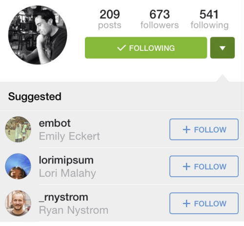
As important as suggestions are to activate new accounts and help them connect to their friends and interests, very little was being done before the team started. We extended the basic infrastructure to collect the data we needed to calculate the best recommendations, implemented some basic algorithms (mostly informed heuristics) and slowly introduced advanced ranking and machine learning techniques. As we evolved our suggestion systems, new opportunities surfaced and we evolved it into the idea of account pivots, automatically surfacing related recommendations when you follow a user’s profile. Some of this work pushed us to fundamentally change the way we were fetching our data, otherwise we wouldn’t be able to provide a good user experience in terms of reliability and latency. I doubt this would be in our radar if we weren’t doing everything end-to-end.

Analytics

Besides all the user-facing products we help build, our systems provide all of the data being used by our analytics team to assess the healthy of our growth and engagement. We introduced new logging frameworks and a built new systems to collect online and offline data. Obviously, we don’t want to reinvent the wheel so those things were only created because the differences in our technology stacks prevented us from using existing Facebook solutions. Having said that, we made sure to connect our data collection mechanisms to Facebook’s data warehousing systems (e.g., Hive, Presto), saving us a tremendous amount of work.

As the examples above demonstrate, the key to our success so far has been our end-to-end ownership of data problems and their solution. But our secret sauce also includes ruthless prioritization, only hiring people with the right experience to solve the problems we have, and favoring diversity of background so people can teach what they know and learn about the things they don’t know.

Continuity

Growing the team is inevitable no matter how efficient we are and we believe our principles should be able to scale. The main ideas of owning projects end-to-end and not being tied to platforms or temporary initiatives can be used as guidelines in any team or organization. We have started to introduce sub-teams on Datagram and things are going quite well so far with coverage areas divided into broader end-to-end themes like Discovery, Content, and Activation. Sub-teams share technologies and collaborate in multiple projects, which has kept us extremely efficient. Later this summer we are even starting a small Datagram presence in New York with a focus on content ranking across multiple parts of the app. The future is hard to predict, but it looks quite promising!

Rodrigo Schmidt manages Instagram’s data infrastructure engineering team.

Search Architecture

Instagram is in the fortunate position to be a small company within the infrastructure of a much larger one. When it makes sense, we leverage resources to leapfrog into experiences that have taken Facebook ten years to build. Facebook’s search infrastructure, Unicorn, is a social-graph-aware search engine that has scaled to indexes containing trillions of documents. In early 2015, Instagram migrated all search infrastructure from Elasticsearch into Unicorn. In the same period, we saw a 65% increase in search traffic as a result of both user growth and a 12% jump in the number of people who are using search every time they use Instagram.

These gains have come in part from leveraging Unicorn’s ability to rank queries using social features and second-order connections. By indexing every part of the Instagram graph, we powered the ability to search for anything you want - people, places, hashtags, media - faster and more easily as part of the new Search and Explore experience in our 7.0 update.

What Is Search?

Instagram’s search infrastructure consists of a denormalized store of all entities of interest: hashtags, locations, users and media. In typical search literature these are called documents. Documents are grouped together into sets which can be queried using extremely efficient set operations such as AND, OR and NOT. The results of these operations are efficiently ranked and trimmed to only the most relevant documents for a given query. When an Instagram user enters a search query, our backend encodes it into set operations and then computes a ranked set of the best results.

Getting Data In

Instagram serves millions of requests per second. Many of these, such as signups, likes, and uploads, modify existing records and append new rows to our master PostgreSQL databases. To maintain the correct set of searchable documents, our search infrastructure needs to be notified of these changes. Furthermore, search typically needs more information than a single row in PostgreSQL — for example, the author’s account vintage is used as a search feature after a photo is uploaded.

To solve the problem of denormalization, we introduced a system called Slipstream where events on Instagram are encoded into a large Thrift structure containing more information than typical consumers would use. These events are binary-serialized and sent over an asynchronous pub/sub channel we call the Firehose. Consumers, such as search, subscribe to the Firehose, filter out irrelevant events and react to remaining events. The Firehose is implemented on top of Facebook's Scribe which makes the messaging process asynchronous. The figure below shows the architecture:

Since Thrift is schematized, we re-use objects across requests and have consumers consume messages without the need for custom deserializers. A subset of our Slipstream schema, corresponding to a photo like is shown below:

struct User {
1: required i64 id;
2: string username;
3: string fullname;
4: bool is_private;
...
}
struct Media {
1: required i64 id; 
2: required i64 owner_id;
3: required MediaContentType content_type;
...
}
struct LikeEvent {
1: required i64 liker_id;
2: required i64 media_id;
3: required i64 media_owner_id;
4: Media media;
5: User liker;
6: User media_owner;
...
8: bool is_following_media_owner;
}
union InstagramEvent {
...
2: LikeEvent like;
...
}
struct FirehoseEvent {
1: required i64 server_time_millis;
2: required InstagramEvent event;
}

Firehose messages are treated as best-effort and a small percentage of data loss is expected in messaging. We establish eventual consistency in search by a process of reconciliation or a base build. Each night, we scrape a snapshot of all Instagram PostgreSQL databases to Hive for data archiving. Periodically, we query these Hive tables and construct all appropriate documents for each search vertical. The base build is merged against data derived from Slipstream to allow our systems to be eventually consistent even in the event of data loss.

Getting Data Out

Processing Queries

Assuming that we have ingested our data correctly, our search infrastructure enables an efficient path to extracting relevant documents given a constraint. We call this constraint a query,

which is typically a derived form of user-supplied text (e.g. “Justin” with the intent of searching for Justin Bieber). Behind the scenes, queries to Unicorn are rewritten into S-Expressions that express clear intent, for example:

(and
user:maxime
(apply followed_by: followed_by:me)
)

which translates to “people named maxime followed by people I follow”. Our search infrastructure proceeds in two (intermixed) steps:

Candidate generation: finding a set of documents that match a given query. Our backend dives into a structure called a reverse index, which finds sets of document ids indexed by a term. For example, we may find the set of users with the name “justin” in the “name:justin” term.

Ranking: choosing the best documents from all the candidates. After getting candidate documents, we look up features which encode metadata about a document. For example, one feature for the user justinbieber would be his number of followers (32.3MM). These features are used to compute a “goodness” score, which is used to order the candidates. The “goodness” score can be either machine learned or hand-tuned — in the machine learning case, we may engineer features that discriminate for clicks or follows to a given candidate.

The result of the two steps is an ordered list of the best documents for a given query.

Graph-Aware Searches

As part of our search improvements, Instagram now takes into account who you follow and who they follow in order to provide a more personalized set of results. This means that it is easier for you to find someone based on the people you follow.

Using Unicorn allowed us to index all the accounts, media, hashtags and places on Instagram and the various relationships between these entities. For example, by indexing a user’s followers, Unicorn can provide answers to questions such as:

“Which accounts does User X follow and are also followed by user Y”

Equally, by indexing the locations tagged in media Unicorn can provide responses for questions such as:

“Media taken in New York City from accounts I follow”

Improving Account Search

While utilizing the Instagram graph alone may provide signals that improve the search experience, it may not be sufficient to find the account you are looking for. The search ranking infrastructure of Unicorn had to be adapted to work well on Instagram.

One way we did this was to model existing connections within Instagram. On Facebook, the basic relationship between accounts is non-directional (friending is always reciprocal). On Instagram, people can follow each other without having to follow back. Our team had to adapt the search ranking algorithms used to store and retrieve account to Instagram’s follow graph. For Instagram, accounts are retrieved from unicorn by going through different mixes of:

“people followed by people you follow”

and

“People followed by people who follow you”

In addition, on Instagram, people can follow each other for various reasons. It doesn’t necessarily mean that a user has the same amount of interest in all the accounts they follow. Our team built a model to rank the accounts followed by each user. This allows us to prioritize showing people followed by people that are more important to the searcher.

A Unified Search Box

Sometimes, the best answer for a search query can be a hashtag or a place. In the previous search experience, Instagram users had to explicitly choose between searching for accounts or hashtags. We made it easier to search for hashtags and places by removing the necessity to select between the different types of results. Instead, we built a ranking framework that allows us to predict which type of results we think the user is looking for. We found in tests that blending hashtags with accounts was such a better experience that clicks on hashtags went up by more than 20%! This increase fortunately didn’t come at the cost of significantly impacting account search.

Our classifiers are both personalized and machine-learned on the logs of searches that users are doing on Instagram. The query logs are aggregated per country to determine if a given search term such as “#tbt” would most likely result in a hashtag search or an account search. Those signals are combined with other signals, such as past searches by a given user and the quality of the results available to show, in order to produce a final blended list of results.

Media Search

Instagram’s search infrastructure is used to power discovery features far away from user-input search. Our largest search vertical, media, contains the billions of posts on Instagram indexed by the trillions of likes. Unlike our other tiers, media search is purely infrastructure — users never enter any explicit media search queries in the app. Instead, we use it to power features that display media: explore, hashtags, locations and our newly launched editorial clusters.

Candidate Generation

Lacking an explicit query, we get creative with our media reverse index terms to enable slicing along different axes. The table below shows a list of some term types currently supported in our media index:

Within each posting list, our media is ordered (“statically ranked”) reverse-chronologically to encourage a strong recency bias for results. For example, we can serve the Instagram’s profile page for @thomas with a single query: (term owner:181861901). Extending to hashtags, we can serve recent media from #hyperlapse through (term hashtag:#hyperlapse). Composing Unicorn’s operators enable us to find @thomas’ Hyperlapses, by issuing (and hashtag:#hyperlapse owner:181861901).

Many of terms exist to encourage diversity in our search results. For example, we may be interested in making sure that some #hyperlapse candidates are posted by verified accounts. Through the use of Unicorn’s WEAK AND operator we can guarantee that at least 30% of candidates come from verified accounts:

(wand 
(term hashtag:#hyperlapse)
(term verified:1 :optional-weight 0.3)
)

We exploit diversity to serve better content in the “top” sections of hashtags and locations.

Features

Although postings lists are ordered chronologically we often want to surface the top media for a given query (hashtag, location, etc.). After candidate generation, we go through a process of ranking which chooses the best media by assigning a score to each document. The scoring function consumes a list of features and outputs a score representing the “goodness” of a given document for our query.

Features in our index can be divided broadly into three categories:

Visual: features that look at the visual content of the image itself. Concretely, we run each of Instagram’s photo through a deep neural net (DNN) image classifier in an attempt to categorize the content of the photo. Afterwards, we perform face detection in order to determine the number and size each of the faces in the photo.
Post metadata: features that look at non-visual content of a given post. Many Instagram posts contain captions, location tags, hashtags and/or mentions which aid in determining search relevancy. For example, the FEATURE_IG_MEDIA_IS_LOCATION_TAGGED is an indicator feature determining whether a post contains a location tag.
Author: features that look at the person who made a given post. Some of the richest information about a post is determined by the person that made it. For example, FEATURE_IG_MEDIA_AUTHOR_VERIFIED is an indicator feature determining whether the author of a post is verified.

Depending on the use case, we tune features weights differently. On the “top” section of location pages we may wish to differentiate between photos of a location and photos in a location and down-rank photos containing large faces. Instagram uses a per-query-type ranking model that allows for modeling choices appropriate to a particular app view.

Case study: Explore

Our media search infrastructure also extends itself into discovery, where we serve interesting content that users aren’t explicitly looking for. Instagram’s Explore Posts feature showcases interesting content from people near to you in the Instagram graph. Concretely, one source of explore candidates “photos liked by people whose photos you have liked”. We can can encode this into a single unicorn query with:

(apply liker:(extract owner: liker:<userid>))

This proceeds inwards-outwards by:

liker:<userid>: posts that you’ve liked
(extract owner:...): the owner of those posts
(apply liker:..): media liked by those owners

After this query generates candidates, we are able to leverage our existing ranking infrastructure to determine the top posts for you. Unlike top posts on hashtag and location pages, the scoring function for explore is machine-learned instead of hand tuned.

Acknowledgements

By Maxime Boucher and Thomas Dimson

This project wouldn’t be possible without the contributions of Tom Jackson, Peter DeVries, Weiyi Liu, Lucas Ou-Yang, Felipe Sodre da Silva and Manoli Liodakis

Trending at Instagram

With last week’s Search and Explore launch, we introduced the ability to easily find interesting moments on Instagram as they happen in the world. The trending hashtags and places you see in Explore surface some of the best, most popular content from across the community, and pull from places and accounts you might not have seen otherwise. Building a system that can parse over 70m new photos each day from over 200m people was a challenge. Here’s a look at how we approached identifying, ranking and presenting the best trending content on Instagram.

Definition of a Trend

Intuitively, a trending hashtag should be one that is being used more than usual, as a result of something specific that is happening in that moment. For example, people don’t usually post about the Aurora Borealis, but on the day we launched, a significant group of people was sharing amazing photos using the hashtag #northernlights. You can see how usage of that hashtag increases over time in the graph below.

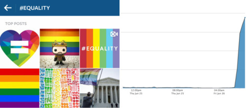
And as we wrote this blog post, #equality was the top trending hashtag on Instagram.

Similarly, a place is trending whenever there is an unusual number of people who share photos or videos taken at that place in a given moment. As we were writing this, the U.S. Supreme Court was also trending, as there were hundreds of people physically there sharing their support of the recent decision in favor of same-sex marriage.

Given examples such as the above, we identified three main elements of a good trend:

Popularity – the trend should be of interest to many people in our community.
Novelty – the trend should be about something new. People were not posting about it before, or at least not with the same intensity.
Timeliness – the trend should surface on Instagram while the real event is taking place.

In this post we discuss the algorithms we use and the system we built to identify trends, rank them and show them in the app.

Identifying a Trend

Identifying a trend requires us to quantify how different the currently observed activity (number of shared photos and videos) is compared to an estimate of what the expected activity is. Generally speaking, if the observed activity is considerably higher than the expected activity, then we can determine that this is something that is trending, and we can rank trends by their difference from the expected values.

Let’s go back to our #equality example in the beginning of this post. Regularly, we observe only a few photos and videos using that hashtag on an hourly basis. For #equality, starting at 07:00AM PT, thousands of people shared content using that hashtag. That means that activity in #equality was well above what we expected. Conversely, more than 100k photos and videos are tagged with #love every day, as it is a very popular hashtag. Even if we observe 10k extra posts in a day, it won’t be enough to exceed our expectations given its historical counts.

For each hashtag and place, we store counters of how many pieces of media were shared using the hashtag or place in a five-minute window over the past seven days. For simplicity, let us focus on hashtags for now, and let’s assume that C(h, t) is the counter for hashtag h at time t (i.e., it is the number of posts that were tagged with this hashtag from time t-5min to time t). Since this count varies a lot between different hashtags and over time, we normalize it and compute the probability P(h, t) of observing the hashtag h at time t. Given the historical counters of a hashtag (aka the time series), we can build a model that predicts the expected number of observations: C’(h, t), and similarly, compute the expected probability P’(h, t). Given these two values for each hashtag, a common measure for the difference between probabilities is the KL divergence, which in our case is computed as:

S(h, t) = P(h, t) * ln(P(h, t)/P’(h, t))

Essentially, we consider both the currently observed popularity, which is captured by P(h, t), and the novelty, computed as the ratio between our current observations and the expected baseline, P(h, t)/P’(h, t). The natural log (ln) function is used to smooth the “strength” of novelty and make it comparable to the popularity. The timeliness role is played by the t parameter, and by looking at the counters in the most recent time windows, trends will be picked up in real-time.

A Prediction Problem

How do you compute the expected baseline probability given past observations?

There are several facets that can influence the accuracy of the estimate and the time-and-space complexity of the computation. Usually those things don’t get along too well - the more accurate you want to be, the more time-and-space complexity the algorithm requires. We experimented with a few different alternatives, like simply taking the count of the same hour last week, and also regression models up to crazy all-knowing neural networks. Turns out that while fancy things tend to have better accuracy, simple things work out well, so we ended up with selecting the maximal probability over the past week’s worth of measurements. Why is this good?

Very easy to compute and relatively low memory demand.
Quite aggressive about suppressing non-trends with high variance.
Quickly identifies emerging trends.

There are two things we over-simplified in this explanation, so let us refine our model a bit more.

First, while some hashtags are extremely popular and have lots of media, most of the hashtags are not popular, and the five-minute counters are extremely low or zero. Thus, we keep an hourly granularity for older counts, as we don’t need a five-minute resolution when computing the baseline probability. We also look at a few hours worth of data so that we can minimize the “noise” caused by random usage spikes. We noted there is a trade-off between the need to get sufficient data and how quickly we can detect trends - the longer the timeframe is, the more data we have, but the slower it will be to identify a trend.

Second, if the predicted baseline P(h, t) is still zero, even after accumulating a few hours for each hashtag, we will not be able to compute the KL divergence measure (division by zero). Hence we apply smoothing, or put more simply: If we didn’t see any media for a given hashtag in the past, we mark it as if we saw three posts in that timeframe. Why three exactly? That allows us to save a large amount of memory (>90%) while storing the counters, as the majority of hashtags do not get more than three posts per hour, so we can simply drop the counters for all of those and assume every hashtag starts with at least three posts per hour.

Ranking and Blending

The next step is to rank the hashtags based on their “trendiness,” which we do by aggregating all the candidate hashtags for a given country/language (the product is enabled in the USA for now) and sorting them according to their KL divergence score, S(h, t). We noticed that some trends tend to disappear faster than the interest around them. For instance, the amount of posts using a hashtag that is trending at the moment will naturally decrease as soon as the event is finished. Therefore, its KL score will quickly decrease, then the hashtag won’t be trending anymore, even though people usually like to see photos and videos from the underlying event of a trend for a few hours after it is over.

In order to overcome those issues, we use an exponential decay function to define the time-to-live for previous trends, or how long we want to keep them for. We keep track of the maximal KL score for each trend, say SM(h), and the time tmax where S(h, tmax) = SM(h). Then, we also compute the exponential decayed value for SM(h) for each candidate hashtag at the moment so that we can blend it with their most recent KL scores.

Sd(h, t) = SM(h) * (½)^((t - tmax)/half-life)

We set the decay parameter half-life to be two hours, meaning that SM(h) is halved every two hours. This way, if a hashtag or a place was a big trend a few hours ago, it may still show up as trending alongside the most recent trends.

Grouping similar trends

People tend to use a range of different hashtags to describe the same event, and when the event is popular, multiple hashtags that describe the same event might all be trending. Since showing multiple hashtags that describe the same event can be an annoying user experience, we group together hashtags that are “conceptually” the same.

For example, the figure above (kudos to Jason Sundram) illustrates all the hashtags that were used together with #equality. It shows that #equality was trending along with #lovewins, #love, #pride, #lgbt and many others. By grouping these tags together, we can show #equality as the trend, and save the need to sift through all the different tags until reaching other interesting trends.

There are two important tasks that need to be achieved - first, understand which hashtags are talking about the same thing, and second, find the hashtag that is the best representative of the group. There are two challenges here - first we need to capture some notion of similarity between hashtags, and then we need to cluster them in an “unsupervised” way, meaning that we have no idea how many clusters there should be at any given time.

We use the following notion of similarity between hashtags:

Cooccurrences - hashtags that tend to be used together, for example #fashionweek, #dress and #model. Cooccurrences are computed by looking at recent media and counting the number of times each hashtag appears together with other hashtags.
Edit distance - different spellings (or typos) of the same hashtag - for example #valentineday and #valentinesday - these tend not to cooccur because people rarely use both together. Spelling variations are taken care of by using Levenshtein distance.
Topic distribution - hashtags that describe the same event - for example #gocavs, #gowarriors - these have different spelling and they are not likely to cooccur. We look at the captions used with these hashtags and run an internal tool that classifies them into a predefined set of topics. For each hashtag we look at the topic distribution (collected from all the media captions in which it appeared) and normalize it using TF-IDF.

Our hashtag grouping process computes the different similarity metrics for each pair of trending hashtags, and then decides which two are similar enough to be considered the same. During the merging process, clusters of tags emerge, and often these clusters will also be merged if they are sufficiently similar.

Now that we have talked about the process for identifying trends at Instagram, let us take a look at how the backend was implemented in order to incorporate each component described above.

System Design

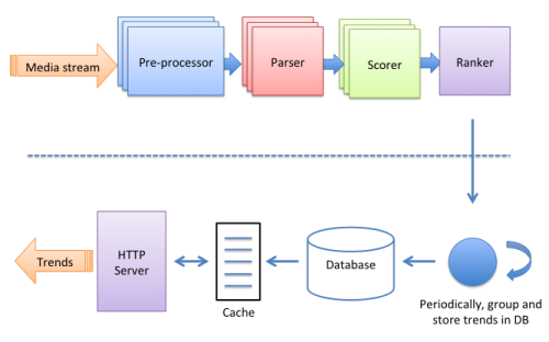
Our trending backend is designed as a stream processing application with four nodes, which are connected in a linear structure like an assembly line, as depicted in the following diagram:

Each node consumes and produces a stream of “log” lines. The entry point receives a stream of media creation events, and the last node outputs a ranked list of trending items (hashtags or places). Each node has a specific role as follows:

pre-processor - the original media creation events holds metadata about the content and its creator, and in the pre-processing phase we fetch and attach to it all the data that is needed in order to apply quality filters in the next step.
parser - extracts the hashtags or place used in a photo or video and applies quality filters. If a post violates our standards, it is not counted towards trending.
scorer - stores time-aggregated counters for each trend. This is also where our scoring function S(h, t) is computed. Every few minutes, a line with the current value for S(h, t) is emitted.
ranker - aggregates and ranks all the candidate trends and their trending scores.

Our system processes and stores a large amount of data in real-time, which should be efficient and tolerant to failures. This stream-lined architecture enables us to partition the trends and launch multiple instances of each node, such that each node stores a smaller amount of data, and the trends are processed in parallel. Furthermore, failures are isolated to specific partitions, so if one instance fails, trending would not be entirely compromised.

So far, we discussed the process that computes trends. The following diagram adds the components that are responsible for serving trends to requests comping from the app:

As the diagram illustrates, requests coming from the Instagram apps for trending hashtags and places need to be served without imposing load on our trending backend. Therefore, trends are served from a read-through caching layer powered by memcached, and a Postgres database, in case there is a cache miss. The database is populated with fresh trends by a periodical task that pulls trends from the ranker, performs the algorithm to group similar trends together and stores the result in Postgres. This way, the Instagram app is always served with the latest trends from our caching layer, which enables us to scale our storage and our stream processing infrastructures independently.

Conclusion

When we approached trending, we tried to break this project down into smaller problems that could be tackled separately by components with a very specific function. As a result, each individual on our team was able to focus on one problem at a time before moving onto the next one. We hope the community will enjoy this update, and be able to better connect to the world as it happens.

By Danilo Resende and Udi Weinsberg

This project wouldn’t be possible without the contributions of Maxime Boucher, Thomas Dimson, David Lee, George Sebastian, Bogdan State and Bai Xiao.

C++ Futures at Instagram

Over the past few months, we’ve built two high-performing recommendation services that handle tens of thousands of queries per second and generate tens of millions connections per day. In this blog post, we want to share our experience of scaling these two services using Futures and, most importantly, how we fine-tuned the details.

The first recommendation service is “Suggested Users.” The SU service fetches candidate accounts from various sources, such as your friends, accounts that you may be interested in, and popular accounts in your area. Then, a machine learning model blends them to produce a list of personalized account suggestions. It powers the people tab on explore, as well as one of the entry points after new users sign up. It is an important means of people discovery on Instagram and generates tens of millions follows per day.

The second service is “Chaining.” Chaining generates a list of accounts that a viewer may be interested in during every profile load. The performance of this service is important - it must be ready to be hit for every profile visit, which translates to over 30,000 queries per second.

These two services share similar infrastructure: they need to make outbound network calls to retrieve suggestions from various sources, load features and rank them before returning them to our Django backend for instrumentation and filtering:

The Thrift threading model

While most of our backend logic lives in Django, we write the services that generate and rank suggestions in C++ using fbthrift. To understand the evolution of our services’ threading model, we need to understand the life cycle of a thrift request. An fbthrift server has three kinds of threads: acceptor threads, I/O threads and worker threads.

When a request comes in:

An acceptor thread accepts the client connection and assigns it to an I/O thread;
The I/O thread reads the input data sent by a client, and passes it to a worker thread and the I/O thread will again be responsible for sending outbound requests later;
The worker thread deserializes the input data into parameters, calls the request handler of the service in its context and spawns additional threads for outbound calls or computation.

The important part is that the thrift request handler runs in a worker thread and not in an I/O thread. This allows the server to be responsive to clients - even if all the worker threads are busy, the server will still have free I/O threads to send an overloaded response to clients and close sockets.

Synchronous I/O: The initial version

The initial version of the service loaded candidates and features synchronously. To reduce latency, all the I/O calls were issued in parallel in separate threads. At the end of the handler was a join() primitive which blocked until all the threads were done. What this essentially means is that one worker thread could only service one client request at a time, and one single request would block as many threads as the number of outbound calls.

This has several disadvantages:

It leads to a large memory footprint - each thread by default has a stack size of several MBs.
We need a separate worker thread to service each client request (and more threads created in the handler to make the I/O calls in parallel). If each request makes M outbound calls, we will have O(M * N) threads waiting for responses.
Thread scheduling also becomes a bottleneck in the kernel at around 400 threads.
With this model, we had to run several hundred instances of server across many machines to support our QPS, because we are not utilizing CPU resource or memory efficiently.

Clearly, there was room for improvement.

Using non-blocking I/O

The fbthrift offers three ways to handle requests: synchronous, asynchronous and future-based. The latter two offer non-blocking I/O and this is how it works : every I/O thread has a list of file descriptors on whose status change it waits on in an event loop (it detects this status change through the select()/poll()/epoll() system call). When the status of the file descriptor changes to “completed,” the I/O thread calls the associated callback. In order to do non-blocking I/O under this mechanism, two things need to be specified:

A callback which will be called when the I/O is complete
The I/O thread whose list should hold the file descriptor corresponding to your I/O operation (This is done by specifying an event base).

This is a typical event-driven programming system. It gives us many nice things:

Waiting on select()/poll()/epoll() puts a thread to sleep, which means it does not busy wait. Thus, it is efficient. To be clear, the synchronous I/O does not necessarily busy wait either, but it requires allocating one thread per I/O call.
One I/O thread can take care of the I/O of multiple outbound requests. This reduces the memory footprint and synchronization costs associated with a large number of threads, and leads to a more scalable system.
One worker thread does not need to wait for all the I/O associated with a single client request to complete before moving on to the next client request. Thus, one worker thread can perform computation for multiple concurrent client requests. Once again, this gives us the benefits mentioned in 2.

Futures : A better asynchronous - programming paradigm

At this point, we were in a pretty good shape in terms of scalability. However, the callback based programming syntax has many deficiencies. For one, it leads to code growing sideways when callbacks are nested, something known as the “callback pyramid.”

doIO1([..](Data io1Result){ doIO2([..](Data io2Result) { doIO3([..](Data io3Result){ .... }, io2Result) }, io1Result) }, io1Input)

This has an impact on code readability and maintainability, and we needed a different async programming paradigm. Two other paradigms are very popular at Facebook - the async/await paradigm used in Hack, which is similar to generators, and the Futures paradigm (through the folly::Futures open-source framework). Futures improve upon the callback-based paradigm with their ability to be composed and chained together. For example, the above code can be written as follows in this paradigm:

doIO1(io1Input) .then([..](Data io1Result) { return doIO2(io1Result); }) .then([..](Data io2Result){ return doIO3(io2Result); }) .then([..](Data io3Result){ ... }) .onError([](const std::exception& e){ // handle errors in io1, io2 or io3 })

This is an example of futures chaining. This solves the ‘callback pyramid’ problem, and makes the code much more readable. It provides the ability to combine Futures together, and also provides very nice error handling mechanisms. (Checkout the github for more examples and features of this API.)

Offloading handler execution from I/O threads

After moving to Futures, we had a performant system with clear, readable code. At this point, we did some profiling to find opportunities for fine-tuning and improvement. One curious thing we noticed was that there was significant delay between the completion of the I/O calls and starting the execution of the 'then’ handler. In fact, the callbacks in the Future chain above are executed in I/O thread contexts, and some of the work they do is non-trivial. This is the source of bottleneck - I/O threads are limited in number and are meant to service I/O status changes. Executing handlers in their context meant that they could not respond to I/O status changes fast enough, causing the delay in execution of handlers. Meanwhile, the worker threads were sitting idle, leading to low CPU utilization. The solution was simple - execute handlers in the context of worker threads. Fortunately, the Futures API provides a very nice interface to achieve this:

doIO1(io1Input) .then(getExecutor() , [..](Data io1Result){ // Do work })

This relieves I/O threads of actual computation such as ranking and reduced our I/O threads busy time by 50%. In addition, this helps prevent cascading failures where I/O threads are all busy and thus none of the callbacks are executed fast enough, which causes most of the requests time out.

Conclusion

With folly Futures, our services can fully exploit system resources and are more reliable and efficient than the ones with synchronous I/O.

We were able to increase the peak CPU utilization of the Suggested User service from 10-15% to 90% per instance. This enabled us to reduce the number of instances of the Suggested Users service from 720 to 38.

Chaining achieved 40 ms average end-to-end latency and under 200ms p99, handling more than 30,000 queries per second. It runs on only 38 instances (each instance handles around 800 requests per second).

By Zhenghao Qian and Gautam Sewani, Software Engineers on the Instagram Data Team

Thanks to Sourav Chatterji, Thomas Dimson, Michael Gorven and Facebook Wangle Team - they all have made great contributions to this effort.

Emojineering Part 2: Implementing Hashtag Emoji

Today’s post is a continuation of Part 1 on emoji semantics.

🙀🔝Last week, Instagram began supporting emoji characters inside of hashtags. On Friday we talked about the rise in emoji usage on Instagram and how to discover the semantics of text. Today’s post will focus on the engineering details of implementing emoji hashtags — a seemingly simple regular expression change that turned into a scary journey through the dark depths of unicode👺.

Where Do Hashtags Come From?

When a caption or comment is added to a photo, Instagram’s server parses hashtags using a regular expression and then indexes the media by hashtag. The regular expression is shared across our clients (Web, Android, iOS), which uses it to link-ify tags in captions and comments.

Before emoji hashtags the Instagram tag regular expression looked something like this:

(?<<<<!>&)#(\w+)

Where \w matches all word-like characters. Seemingly, we just need to add valid emoji characters to the list, deploy new Instagram binaries, and then call it a day 😏. In reality, it turns out even a simple regular expression change can be 😲 crazy-complicated.

Background on Unicode

To fully understand this post, you will need a minimal background on Unicode. Here’s a quick overview.

Within Unicode, characters (the Roman alphabet, cyrillic characters, emoji, etc.) are represented using various code points, or numbers. Characters of different languages are enumerated in a standard called Unicode. Computers express these numbers using various encodings. Most software engineers need to know about 3:

UTF-8: Expresses unicode code points as a variable-length sequence of bytes. Characters in low code point ranges, like english text, can be expressed in a single byte, while characters in higher ranges could take up to four.
UTF-16: Also expresses unicode code points as a variable-length sequence of bytes. These sequences are either two bytes (for lower code point ranges) or four bytes (for higher code point ranges). Higher ranges are encoded in using two 16-bit units called “surrogate pairs.”
UTF-32: Expresses unicode code points consistently as a four-byte sequence.

UTF-16 is one of the most complex encodings because of the presence of surrogate pairs. Unfortunately, it is also the native encoding for Objective-C, Java and Python (2.x series under certain compiler flags).

A First Attempt

Instagram has an engineering philosophy of doing the simple thing first. I started by reading the Wikipedia article on emoji, which lead me to believe that all emoji are single unicode code points in one of five unicode blocks: Miscellaneous Symbols and Pictographs, Emoticons, Transport and Map Symbols, Miscellaneous Symbols and Dingbats. Naively, I wrote a regular expression that matched each range individually. Something like:

[\U0001F300-\U0001F5FF\U0001F600-\U0001F64F\U0001F680-\U0001F6FF\u2600-\u26FF\u2700–\u27BF]

While testing on iOS, I was able to tag some of my favorite emoji like 💩and 🍦. Unfortunately some deeper testing violated my assumptions…

What Goes Wrong and the TR51 Draft Standard

❤️ didn’t work. 🇺🇸 didn’t work. Even the arrow emoji ⬆️➡️⬇️⬅️ didn’t work. As I found out, it doesn’t suffice to match particular character emoji ranges because:

Some emoji consist of multiple code points in Unicode. For example, flag emojis consist of two code points, spelling out country abbreviations from the ISO 3166-1 standard. While iOS hasn’t implemented the Greenlandic flag, you can still express it using the letters G and L.
The iOS emoji keyboards express some emoji in so-called variant forms. An emoji like ❤️ will be expressed using one code point corresponding to the heart, followed by a variant selector code point, which chooses a particular glyph to represent the heart. In theory, there can be up to 16 variant forms for any single-code-point emoji. Some emoji lie outside those unicode blocks. For example, the CJK ideographs 🈹🈶🈵🈳Emoji aren’t yet standardized, and finding these problems consists of a lot of trial and error.

Fortunately, I came across the TR51 Draft Technical Report on Emoji which documents most of the variants present across iOS and Android. The draft even comes with a series of data files which list the common emoji on iOS and Android.

Generating Regular Expressions with Code

The TR51 draft has 1,245 emoji listed which rules out hand-writing a regular expression. Instead, I wrote a script which parses code points out of the list and constructs a minimal regular expression using character ranges. For languages like Objective-C the approach works wonderfully. Unfortunately Instagram’s server runs Python 2.7 which leaks some internal character-encoding details outwards.

Encoding Differences: Taking Python into the Astral Plane ♉️

Python 2.x can be compiled in both wide-mode (using UTF-32 internally) or narrow-mode (using UTF-16 internally). As discussed, UTF-16 represents characters from high code point ranges (humorously known as the Astral Plane) using a pair of two-byte sequences called surrogate pairs. In narrow Python builds, four-byte unicode escapes are not allowed as regular expression character ranges. Thus, instead of matching the emoticon block using something sane like:

[\U0001F600-\U0001F64F]

We have to use a non-range surrogate pair match like:

(\uD83D[\uDE00-\uDE4F])

😭😭😭

Syntax Differences

😳The regular expression for Instagram hashtags spans many codebases including our clients (Java, Javascript, Objective-C), server (Python), and data (HiveQL, C++). Unicode escaping works subtly differently across languages forcing our regular expression generation script to have multiple outputs. Of particular note: Java 7 was the first release to include escaping for astral plane unicode characters. The escaping syntax is only valid in regular expressions and can’t be used to escape strings. For example, you can match U+0001F600 with the pattern \x{1F600}. Since this is a new feature not available in all Android versions, we compile the pattern within a try {} catch {} block, falling back to a legacy list of low-range emoji on failure.

Objective-C supports unicode escaping for astral plane characters in strings with \U0001F600. Unfortunately, the syntax doesn’t work in the ASCII range, forcing a mixture of another \xf6 syntax. Certain printable characters aren’t allowed to be specified with a hex sequence and require direct embedding into a string.

ECMAscript (Javascript) versions prior to 6 has the same surrogate pair and two-byte escaping problems of Python resulting in a similar regular expression.

Pattern Matching Differences

What does \w mean in a regular expression? In an ASCII world \w matches latin “word” characters but in a Unicode world the UTS 18 technical standard recommends that \w matches digits, alphabetical characters, the general category of “mark,” and two categories called “Connector Punctuation” and “Join Control.” The latter two categories are used in some emoji but programming languages implement it differently. Objective-C on iOS 8.3 will match \w against U+200d and U+fe0f. Python matches neither. Peculiarly, the Java JRE (8.0) matches neither while the Android Java runtime (API level 16) matches only U+fe0f.

Thus, depending on the platform we have to augment the allowed character set to include special non-printable characters 👎

iOS 8.3’s New Emoji

iOS 8.3 came out during our hashtag emoji development and brought new types to the mix. In particular, Apple gave us a wide variety of skin tone and family options. Both of them require multiple Unicode code points, requiring more optional characters at the end of regular expressions:

Skin tone options 🎅🏻🎅🏼🎅🏽🎅🏾🎅🏿. iOS brings skin tone options to existing emoji such as Santa Claus (U+1F385). They are implemented by pairing up the emoji with a skin tone “fitzpatrick” character from the range U+1F3FB-U+1F3FF. Due to the implementations, older releases and other platforms will render the emoji as two separate characters (🎅,🏻).
Diverse families 👩‍👩‍👧‍👦 . iOS brings support for many different family variants (sex, number of children). They are implemented as separate unicode code points for each member of the family, joined together with the unicode U+200D zero-width joiner character. This means that family emoji are implemented with up to 7 unicode code points that literally spell each member of the family: woman-woman-girl-boy. On older releases and other platforms, you will see each family member individually (👩,👩,👧,👦)
Diverse kisses 👨‍❤️‍💋‍👨. Similar to diverse families, kisses between same-sex couples are implemented using five unicode code points joined together with U+200D. These kiss emoji literally spell out one kisser, a heart emoji with a variant selector character, the lips emoji and then the other kisser. On older releases and other platforms, you will see each part spelled out explicitly (👨‍,❤️‍,💋‍,👨)

Modeling Decisions

Emoji variants bring up some difficult modeling questions around what constitutes a hashtag. To date, Instagram has created a new hashtag for each distinct Unicode sequence. But what about emoji variants? Should photos under 🎅🏻be indexed under 🎅? Should it be possible to mix non-emoji characters with emoji?

Starting from the simple thing first, we felt it may be surprising for posters to see #🎅🏻 photos under #🎅 and so we indexed them separately. If we need to change our decision, it is easier to consolidate variants under a single parent than it is to break the parent into difference pieces.

We went back and forth on whether to allow mixing of emoji and script together. While allowing richer expression, it also creates edge cases when appending emoji to the end of existing hashtags like #tbt👎. After playing with emoji tags around the office, we sided with expression. How else can you express #dealwithit😎 ?

The Result✔️

Armed with the knowledge of syntax variants, selector characters, skin tone options, modeling decisions, and UTF-16 wackiness, we are in a position write a script that produces correct regular expressions across all platforms. In the end, Instagram uses regular expressions such as:

Python 2.7

Java 7+

"(?<!&)#(\w|[\\x{2712}\\x{2714}\\x{2716}\\x{271d}\\x{2721}\\x{2728}\\x{2733}\\x{2734}\\x{2744}\\x{2747}\\x{274c}\\x{274e}\\x{2753}-\\x{2755}\\x{2757}\\x{2763}\\x{2764}\\x{2795}-\\x{2797}\\x{27a1}\\x{27b0}\\x{27bf}\\x{2934}\\x{2935}\\x{2b05}-\\x{2b07}\\x{2b1b}\\x{2b1c}\\x{2b50}\\x{2b55}\\x{3030}\\x{303d}\\x{1f004}\\x{1f0cf}\\x{1f170}\\x{1f171}\\x{1f17e}\\x{1f17f}\\x{1f18e}\\x{1f191}-\\x{1f19a}\\x{1f201}\\x{1f202}\\x{1f21a}\\x{1f22f}\\x{1f232}-\\x{1f23a}\\x{1f250}\\x{1f251}\\x{1f300}-\\x{1f321}\\x{1f324}-\\x{1f393}\\x{1f396}\\x{1f397}\\x{1f399}-\\x{1f39b}\\x{1f39e}-\\x{1f3f0}\\x{1f3f3}-\\x{1f3f5}\\x{1f3f7}-\\x{1f4fd}\\x{1f4ff}-\\x{1f53d}\\x{1f549}-\\x{1f54e}\\x{1f550}-\\x{1f567}\\x{1f56f}\\x{1f570}\\x{1f573}-\\x{1f579}\\x{1f587}\\x{1f58a}-\\x{1f58d}\\x{1f590}\\x{1f595}\\x{1f596}\\x{1f5a5}\\x{1f5a8}\\x{1f5b1}\\x{1f5b2}\\x{1f5bc}\\x{1f5c2}-\\x{1f5c4}\\x{1f5d1}-\\x{1f5d3}\\x{1f5dc}-\\x{1f5de}\\x{1f5e1}\\x{1f5e3}\\x{1f5ef}\\x{1f5f3}\\x{1f5fa}-\\x{1f64f}\\x{1f680}-\\x{1f6c5}\\x{1f6cb}-\\x{1f6d0}\\x{1f6e0}-\\x{1f6e5}\\x{1f6e9}\\x{1f6eb}\\x{1f6ec}\\x{1f6f0}\\x{1f6f3}\\x{1f910}-\\x{1f918}\\x{1f980}-\\x{1f984}\\x{1f9c0}\\x{3297}\\x{3299}\\x{a9}\\x{ae}\\x{203c}\\x{2049}\\x{2122}\\x{2139}\\x{2194}-\\x{2199}\\x{21a9}\\x{21aa}\\x{231a}\\x{231b}\\x{2328}\\x{2388}\\x{23cf}\\x{23e9}-\\x{23f3}\\x{23f8}-\\x{23fa}\\x{24c2}\\x{25aa}\\x{25ab}\\x{25b6}\\x{25c0}\\x{25fb}-\\x{25fe}\\x{2600}-\\x{2604}\\x{260e}\\x{2611}\\x{2614}\\x{2615}\\x{2618}\\x{261d}\\x{2620}\\x{2622}\\x{2623}\\x{2626}\\x{262a}\\x{262e}\\x{262f}\\x{2638}-\\x{263a}\\x{2648}-\\x{2653}\\x{2660}\\x{2663}\\x{2665}\\x{2666}\\x{2668}\\x{267b}\\x{267f}\\x{2692}-\\x{2694}\\x{2696}\\x{2697}\\x{2699}\\x{269b}\\x{269c}\\x{26a0}\\x{26a1}\\x{26aa}\\x{26ab}\\x{26b0}\\x{26b1}\\x{26bd}\\x{26be}\\x{26c4}\\x{26c5}\\x{26c8}\\x{26ce}\\x{26cf}\\x{26d1}\\x{26d3}\\x{26d4}\\x{26e9}\\x{26ea}\\x{26f0}-\\x{26f5}\\x{26f7}-\\x{26fa}\\x{26fd}\\x{2702}\\x{2705}\\x{2708}-\\x{270d}\\x{270f}]|\\x{23}\\x{20e3}|\\x{2a}\\x{20e3}|\\x{30}\\x{20e3}|\\x{31}\\x{20e3}|\\x{32}\\x{20e3}|\\x{33}\\x{20e3}|\\x{34}\\x{20e3}|\\x{35}\\x{20e3}|\\x{36}\\x{20e3}|\\x{37}\\x{20e3}|\\x{38}\\x{20e3}|\\x{39}\\x{20e3}|\\x{1f1e6}[\\x{1f1e8}-\\x{1f1ec}\\x{1f1ee}\\x{1f1f1}\\x{1f1f2}\\x{1f1f4}\\x{1f1f6}-\\x{1f1fa}\\x{1f1fc}\\x{1f1fd}\\x{1f1ff}]|\\x{1f1e7}[\\x{1f1e6}\\x{1f1e7}\\x{1f1e9}-\\x{1f1ef}\\x{1f1f1}-\\x{1f1f4}\\x{1f1f6}-\\x{1f1f9}\\x{1f1fb}\\x{1f1fc}\\x{1f1fe}\\x{1f1ff}]|\\x{1f1e8}[\\x{1f1e6}\\x{1f1e8}\\x{1f1e9}\\x{1f1eb}-\\x{1f1ee}\\x{1f1f0}-\\x{1f1f5}\\x{1f1f7}\\x{1f1fa}-\\x{1f1ff}]|\\x{1f1e9}[\\x{1f1ea}\\x{1f1ec}\\x{1f1ef}\\x{1f1f0}\\x{1f1f2}\\x{1f1f4}\\x{1f1ff}]|\\x{1f1ea}[\\x{1f1e6}\\x{1f1e8}\\x{1f1ea}\\x{1f1ec}\\x{1f1ed}\\x{1f1f7}-\\x{1f1fa}]|\\x{1f1eb}[\\x{1f1ee}-\\x{1f1f0}\\x{1f1f2}\\x{1f1f4}\\x{1f1f7}]|\\x{1f1ec}[\\x{1f1e6}\\x{1f1e7}\\x{1f1e9}-\\x{1f1ee}\\x{1f1f1}-\\x{1f1f3}\\x{1f1f5}-\\x{1f1fa}\\x{1f1fc}\\x{1f1fe}]|\\x{1f1ed}[\\x{1f1f0}\\x{1f1f2}\\x{1f1f3}\\x{1f1f7}\\x{1f1f9}\\x{1f1fa}]|\\x{1f1ee}[\\x{1f1e8}-\\x{1f1ea}\\x{1f1f1}-\\x{1f1f4}\\x{1f1f6}-\\x{1f1f9}]|\\x{1f1ef}[\\x{1f1ea}\\x{1f1f2}\\x{1f1f4}\\x{1f1f5}]|\\x{1f1f0}[\\x{1f1ea}\\x{1f1ec}-\\x{1f1ee}\\x{1f1f2}\\x{1f1f3}\\x{1f1f5}\\x{1f1f7}\\x{1f1fc}\\x{1f1fe}\\x{1f1ff}]|\\x{1f1f1}[\\x{1f1e6}-\\x{1f1e8}\\x{1f1ee}\\x{1f1f0}\\x{1f1f7}-\\x{1f1fb}\\x{1f1fe}]|\\x{1f1f2}[\\x{1f1e6}\\x{1f1e8}-\\x{1f1ed}\\x{1f1f0}-\\x{1f1ff}]|\\x{1f1f3}[\\x{1f1e6}\\x{1f1e8}\\x{1f1ea}-\\x{1f1ec}\\x{1f1ee}\\x{1f1f1}\\x{1f1f4}\\x{1f1f5}\\x{1f1f7}\\x{1f1fa}\\x{1f1ff}]|\\x{1f1f4}\\x{1f1f2}|\\x{1f1f5}[\\x{1f1e6}\\x{1f1ea}-\\x{1f1ed}\\x{1f1f0}-\\x{1f1f3}\\x{1f1f7}-\\x{1f1f9}\\x{1f1fc}\\x{1f1fe}]|\\x{1f1f6}\\x{1f1e6}|\\x{1f1f7}[\\x{1f1ea}\\x{1f1f4}\\x{1f1f8}\\x{1f1fa}\\x{1f1fc}]|\\x{1f1f8}[\\x{1f1e6}-\\x{1f1ea}\\x{1f1ec}-\\x{1f1f4}\\x{1f1f7}-\\x{1f1f9}\\x{1f1fb}\\x{1f1fd}-\\x{1f1ff}]|\\x{1f1f9}[\\x{1f1e6}\\x{1f1e8}\\x{1f1e9}\\x{1f1eb}-\\x{1f1ed}\\x{1f1ef}-\\x{1f1f4}\\x{1f1f7}\\x{1f1f9}\\x{1f1fb}\\x{1f1fc}\\x{1f1ff}]|\\x{1f1fa}[\\x{1f1e6}\\x{1f1ec}\\x{1f1f2}\\x{1f1f8}\\x{1f1fe}\\x{1f1ff}]|\\x{1f1fb}[\\x{1f1e6}\\x{1f1e8}\\x{1f1ea}\\x{1f1ec}\\x{1f1ee}\\x{1f1f3}\\x{1f1fa}]|\\x{1f1fc}[\\x{1f1eb}\\x{1f1f8}]|\\x{1f1fd}\\x{1f1f0}|\\x{1f1fe}[\\x{1f1ea}\\x{1f1f9}]|\\x{1f1ff}[\\x{1f1e6}\\x{1f1f2}\\x{1f1fc}])+"

Objective-C

"[\U00002712\U00002714\U00002716\U0000271d\U00002721\U00002728\U00002733\U00002734\U00002744\U00002747\U0000274c\U0000274e\U00002753-\U00002755\U00002757\U00002763\U00002764\U00002795-\U00002797\U000027a1\U000027b0\U000027bf\U00002934\U00002935\U00002b05-\U00002b07\U00002b1b\U00002b1c\U00002b50\U00002b55\U00003030\U0000303d\U0001f004\U0001f0cf\U0001f170\U0001f171\U0001f17e\U0001f17f\U0001f18e\U0001f191-\U0001f19a\U0001f201\U0001f202\U0001f21a\U0001f22f\U0001f232-\U0001f23a\U0001f250\U0001f251\U0001f300-\U0001f321\U0001f324-\U0001f393\U0001f396\U0001f397\U0001f399-\U0001f39b\U0001f39e-\U0001f3f0\U0001f3f3-\U0001f3f5\U0001f3f7-\U0001f4fd\U0001f4ff-\U0001f53d\U0001f549-\U0001f54e\U0001f550-\U0001f567\U0001f56f\U0001f570\U0001f573-\U0001f579\U0001f587\U0001f58a-\U0001f58d\U0001f590\U0001f595\U0001f596\U0001f5a5\U0001f5a8\U0001f5b1\U0001f5b2\U0001f5bc\U0001f5c2-\U0001f5c4\U0001f5d1-\U0001f5d3\U0001f5dc-\U0001f5de\U0001f5e1\U0001f5e3\U0001f5ef\U0001f5f3\U0001f5fa-\U0001f64f\U0001f680-\U0001f6c5\U0001f6cb-\U0001f6d0\U0001f6e0-\U0001f6e5\U0001f6e9\U0001f6eb\U0001f6ec\U0001f6f0\U0001f6f3\U0001f910-\U0001f918\U0001f980-\U0001f984\U0001f9c0\U00003297\U00003299\U000000a9\U000000ae\U0000203c\U00002049\U00002122\U00002139\U00002194-\U00002199\U000021a9\U000021aa\U0000231a\U0000231b\U00002328\U00002388\U000023cf\U000023e9-\U000023f3\U000023f8-\U000023fa\U000024c2\U000025aa\U000025ab\U000025b6\U000025c0\U000025fb-\U000025fe\U00002600-\U00002604\U0000260e\U00002611\U00002614\U00002615\U00002618\U0000261d\U00002620\U00002622\U00002623\U00002626\U0000262a\U0000262e\U0000262f\U00002638-\U0000263a\U00002648-\U00002653\U00002660\U00002663\U00002665\U00002666\U00002668\U0000267b\U0000267f\U00002692-\U00002694\U00002696\U00002697\U00002699\U0000269b\U0000269c\U000026a0\U000026a1\U000026aa\U000026ab\U000026b0\U000026b1\U000026bd\U000026be\U000026c4\U000026c5\U000026c8\U000026ce\U000026cf\U000026d1\U000026d3\U000026d4\U000026e9\U000026ea\U000026f0-\U000026f5\U000026f7-\U000026fa\U000026fd\U00002702\U00002705\U00002708-\U0000270d\U0000270f]|[#]\U000020e3|[*]\U000020e3|[0]\U000020e3|[1]\U000020e3|[2]\U000020e3|[3]\U000020e3|[4]\U000020e3|[5]\U000020e3|[6]\U000020e3|[7]\U000020e3|[8]\U000020e3|[9]\U000020e3|\U0001f1e6[\U0001f1e8-\U0001f1ec\U0001f1ee\U0001f1f1\U0001f1f2\U0001f1f4\U0001f1f6-\U0001f1fa\U0001f1fc\U0001f1fd\U0001f1ff]|\U0001f1e7[\U0001f1e6\U0001f1e7\U0001f1e9-\U0001f1ef\U0001f1f1-\U0001f1f4\U0001f1f6-\U0001f1f9\U0001f1fb\U0001f1fc\U0001f1fe\U0001f1ff]|\U0001f1e8[\U0001f1e6\U0001f1e8\U0001f1e9\U0001f1eb-\U0001f1ee\U0001f1f0-\U0001f1f5\U0001f1f7\U0001f1fa-\U0001f1ff]|\U0001f1e9[\U0001f1ea\U0001f1ec\U0001f1ef\U0001f1f0\U0001f1f2\U0001f1f4\U0001f1ff]|\U0001f1ea[\U0001f1e6\U0001f1e8\U0001f1ea\U0001f1ec\U0001f1ed\U0001f1f7-\U0001f1fa]|\U0001f1eb[\U0001f1ee-\U0001f1f0\U0001f1f2\U0001f1f4\U0001f1f7]|\U0001f1ec[\U0001f1e6\U0001f1e7\U0001f1e9-\U0001f1ee\U0001f1f1-\U0001f1f3\U0001f1f5-\U0001f1fa\U0001f1fc\U0001f1fe]|\U0001f1ed[\U0001f1f0\U0001f1f2\U0001f1f3\U0001f1f7\U0001f1f9\U0001f1fa]|\U0001f1ee[\U0001f1e8-\U0001f1ea\U0001f1f1-\U0001f1f4\U0001f1f6-\U0001f1f9]|\U0001f1ef[\U0001f1ea\U0001f1f2\U0001f1f4\U0001f1f5]|\U0001f1f0[\U0001f1ea\U0001f1ec-\U0001f1ee\U0001f1f2\U0001f1f3\U0001f1f5\U0001f1f7\U0001f1fc\U0001f1fe\U0001f1ff]|\U0001f1f1[\U0001f1e6-\U0001f1e8\U0001f1ee\U0001f1f0\U0001f1f7-\U0001f1fb\U0001f1fe]|\U0001f1f2[\U0001f1e6\U0001f1e8-\U0001f1ed\U0001f1f0-\U0001f1ff]|\U0001f1f3[\U0001f1e6\U0001f1e8\U0001f1ea-\U0001f1ec\U0001f1ee\U0001f1f1\U0001f1f4\U0001f1f5\U0001f1f7\U0001f1fa\U0001f1ff]|\U0001f1f4\U0001f1f2|\U0001f1f5[\U0001f1e6\U0001f1ea-\U0001f1ed\U0001f1f0-\U0001f1f3\U0001f1f7-\U0001f1f9\U0001f1fc\U0001f1fe]|\U0001f1f6\U0001f1e6|\U0001f1f7[\U0001f1ea\U0001f1f4\U0001f1f8\U0001f1fa\U0001f1fc]|\U0001f1f8[\U0001f1e6-\U0001f1ea\U0001f1ec-\U0001f1f4\U0001f1f7-\U0001f1f9\U0001f1fb\U0001f1fd-\U0001f1ff]|\U0001f1f9[\U0001f1e6\U0001f1e8\U0001f1e9\U0001f1eb-\U0001f1ed\U0001f1ef-\U0001f1f4\U0001f1f7\U0001f1f9\U0001f1fb\U0001f1fc\U0001f1ff]|\U0001f1fa[\U0001f1e6\U0001f1ec\U0001f1f2\U0001f1f8\U0001f1fe\U0001f1ff]|\U0001f1fb[\U0001f1e6\U0001f1e8\U0001f1ea\U0001f1ec\U0001f1ee\U0001f1f3\U0001f1fa]|\U0001f1fc[\U0001f1eb\U0001f1f8]|\U0001f1fd\U0001f1f0|\U0001f1fe[\U0001f1ea\U0001f1f9]|\U0001f1ff[\U0001f1e6\U0001f1f2\U0001f1fc]"

Adieu

If you look at three random Instagram comments, chances are that you’ll find emoji. Their usage has rippled across human languages and emoji frequently function as word-substitutes. They are natural choice for supporting in Instagram hashtags but identifying characters can be difficult in across programming languages. Only by parsing the standard, finding character variations, and understanding language differences do they become possible to support.

I’ll see you in the #☁️

Thomas Dimson is a Software Engineer on the Instagram Data Team, and also created Instagram’s Hyperlapse app.

Emojineering Part 1: Machine Learning for Emoji Trends

🆒🆕In October 2011, Apple added the emoji keyboard to iOS as an international keyboard. Since then, digital language has evolved such that nearly half of comments and captions on Instagram contain emoji characters. And earlier this week, Instagram also added support for emoji characters in hashtags, which allows people to tag and search content with their favorite emoji #🎉.

In Part 1 of this blog post series, we will take a deep dive into emoji usage on Instagram. By applying machine learning and natural language processing techniques, we’ll discover the hidden semantics of emoji.

Emoji on Instagram: Up and to the Right

It is a rare privilege to observe the rise of a new language. Instagram has always supported emoji, but they did not see wide adoption until the introduction of the emoji keyboard on iOS (October 2011) and on most Android platforms (July 2013). The graph below shows the percentage of text (comments and captions) containing emoji characters graphed over time 📈.

In the month following the introduction of the iOS emoji keyboard, 10% of text on Instagram contained emoji. The trend continued until the release of Instagram for Android in April of 2012, when many new users did not have emoji support. Afterwards, there was a clear upward trend which accelerated after Android received native support for emoji in July 2013.

Usage continued to grow and in March of this year, nearly half of text contained emoji 😱. In the future, will all text contain emoji? To help answer that question, we divided emoji usage by country and observed the differences between user cohorts.

The graph below shows that users from Finland are using emoji characters in over 60% of text! In contrast, the lower bound is in Tanzania with only 10% of text containing emoji. If the overall trend continues, we might be looking at a future where the majority of text on Instagramcontains emoji.

Natural Language Processing

Learning an Emoji Representation

We’re often asked about the meaning of emoji such as 🙇. Intuitively, substitutable words have similar meanings. For example, we might say that “dog” and “cat” are similar words because they can both be used in sentences like “The pet store sells _ food.” In the field of natural language processing, this intuition is called the distributional hypothesis 🎓. It can be applied to emoji by treating them as if they are normal words.

More formally, we can place (or embed) emoji and hashtags together with words into a common metric space where there are well-defined distances between elements. The representation of the words are chosen so that similar words have a small distance. In the scatter chart below, we embedded words, emoji, and hashtags into a 100-dimensional space of floating point numbers using 50 million English Instagram comments and captions from 2015.

We learn the floating point numbers using the Gensim library, which re-implements a tool called word2vec. In skip-gram mode, word2vec reads through text and predicts the context around a given word or emoji. If the algorithm predicts the context incorrectly, then it adjusts its internals to make a better guess in the next round. As part of that unsupervised training process, word2vec learns our 100-dimensional representation for words and emoji.

Emoji Translations

Having learned a good representation for emoji, we can begin to ask questions about similarity. Namely, for a given emoji, what English words are semantically similar? For each emoji, we compute the “angle” (equivalently the cosine similarity) between it and other words. Words with a small angle are said to be similar and provide a natural, English-language translation for that emoji.

Using our algorithm, we find that many of our popular emoji have meanings in-line with early internet slang:

😂 (ranked 1st in emoji usage): lolol, lmao, lololol, lolz, lmfao, lmaoo, lolololol, lol, ahahah, ahahha, loll, ahaha, ahah, lmfaoo, ahha, lmaooo, lolll, lollll, ahahaha, ahhaha, lml, lmfaooo
😍 (ranked 2nd in emoji usage): beautifull, gawgeous, gorgeous, perfff, georgous, gorgous, hottt, goregous, cuteeee, beautifullll, georgeous, baeeeee, hotttt, babeee, sexyyyy, perffff, hawttt
❤ (ranked 3rd in emoji usage): xoxoxox, xoxoxo, xoxo, xoxoxoxo, xoxoxoxoxo, xoxoxoxox, xxoo, oxox, babycakes, muahhhh, mwahh, babe, boobear, loveyou, bunches, muahhh, muahh, xoxox, muahhhhh
👍(ranked 9th in emoji usage): #keepitup, #fingerscrossed, aswell, haha, #impressed, #yourock, lol, #greatjob, bud, #goodjob, awesome, good, #muchlove, #proudofyou, job, #goodluck
😭(ranked 11th in emoji usage): ughh, ughhh, ughhhh, ugh, uggh, ugghh, ughhhhh, ughhhhhh, ugggh, lolol, wahhhh, rn, oml, uhg, agh, xc, omgg, omfg, omf, lololol, whyyy, loll, wahhhhh, tooo, kms

Some of the more distinctive emoji had particularly distinctive meanings:

🙌: #waitonit, #justwaitonit, #wonthedoit, #nuffsaid, #yeslawd, #youtherealmvp, #stayblessed, #thatisall, thou, #enoughsaid, leggo, #onlythebeginning
👯: #sistasista, #sistersforlife, #sistersister, #bestiesforlife, yearsoffriendship, #sisterfromanothermister, #morelikesisters, #bffl, #bestiesfortheresties, #bestfriendsforever
💃: #birthdaybehavior, #bdaybehavior, #tu, #ladiesnight, #turnuptime, #dontmissit, #bdaycelebration, #piscesseason, #bethere, turnup, #grownandsexy
🎅: merry, christmas, #merrychristmas, #christmas2014, #christmaseve, #christmastime, xmas, eve, #santa, claus, #happyholidays, #xmas, clause, reindeer, pesach

Naturally, people have strong associations with the flag emoji:

🇺🇸 : merica, #godblessamerica, ‘merica, #murica, #merica, #hooah, #america, #specialforces, #supportourtroops, #goarmy, #redwhiteandblue
🇫🇷 : paris, france, #eiffeltower, #paris, #france, louvre, italy, #montreal
🇯🇵 : #japan, #osaka, #kyoto, #japanese, japan, taipei, osaka, beijing, taiwan, tokyo, #日本

And in answer to our question, we can find that the 🙇 emoji is associated with: #goodmorningtho,#yadigg,lbvs,#gn,#inmyfeelings,#latenightthoughts,#deletinglater. Personally, I like laughing but very serious (lbvs).

Changing the vocabulary

It seems that the most popular emoji have similar semantics to words like “lol/hehe” (😂), “xoxo” (❤️) and “omg” (😱). Are these emoji also replacing the usage of the words?

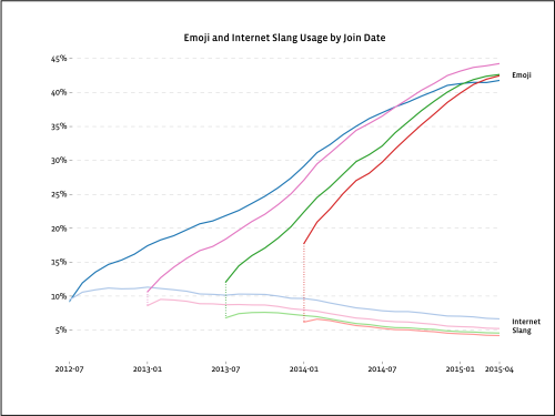
Precisely, we examine the usage of language in Instagram comments and captions by measuring the percentage of text containing emoji or internet slang. To control for natural changes in Instagram demographics, we examined four cohorts past the launch of Instagram for Android: those joining Instagram in the first week of July 2012, January 2013, July 2013, and January 2014. Each cohort contains millions of Instagram users. We defined internet slang as words matching variants of “xoxo”, “omg”, “muah”, “babe”, “bae”, “lol”, “haha,” and “hehe” with the following regular expression:

(?:\b|#)((?:xo)+|omg+|muah+|babe+|bae+|lol+|(?:ha|he)+h?)(\b|\.|!|\?)

As shown in the chart below, all groups exhibit a similar pattern in the rise of emoji (with an upper bound around 45%) and a decline of internet slang (with a lower bound of around 5%). Correlation coefficients within the respective cohorts are all below -0.93, indicating a strongly negative correlation.

The vocabulary of Instagram is shifting similarly across many different cohorts with a decline in internet slang corresponding to rise in the usage of emoji.

The Hearts of Instagram

Having our vectorized representation opens up a wealth of semantic analysis. One of the purported advantages of word2vec representations are that they allow for algebraic operations in semantic space. For example, it can be particularly hard to distinguish the heart emoji 💙💚💛💜💖💗💌. We can isolate some of the effects by subtracting off the representation of ❤️ and finding similar concepts roughly corresponding to color. For example:

💙 - ❤️ ~= #goblue, #letsgoduke, #bleedblue, #ibleedblue, #worldautismawarenessday, #goduke, #beatduke, #autismspeaks, #autismawarenessday, #gobroncos, duke
💚 - ❤️ ~= #gogreen, loyals, #herballife, #happysaintpatricksday, 🍏, #stpats, 🍀, #jointhemovement, green, #hairskinnails, #happystpatricksday
💛 - ❤️ ~= 🌱 ,🍊 ,#springhassprung ,🔆 ,#springiscoming ,#springishere, #aprilshowers, #thinkspring, #hellospring, 🌻, #wildflower, #happyearthday
💜- ❤️~= ✨, 🌀, 🔮, 🌟, 💄, 🎀, faldc, 💎, brassy, topaz, peachy ,purple, #thinkpink,☁, sparkle, 🌿, shimmer, sparkles, kaleidoscope, periwinkle, 🍄, greenish
💖 -❤️ ~= gorl, 💮, cwd, s4s, aynmalik, spvm, ulee, 💧, 🈹, yulema, sfs, bvby, ɑnd, indirect, priv
💗 -❤️ ~= ulitzer, 🎀, peachy, february’s, tulle, mackz, kendall’s, curvy, faldc, #dancewear, strapless, 👗, ◽, floral
💌 - ❤️ ~= 📫, ℹ, 📬, 📮, ✉, 📩, 💳, 💻, 📦, paypal, 📧, item, ⏬, 📱, inquire, orders, payment, 📄, 📋, 📲, deposit

Naturally, there are some mistakes in this type of algebra. Nonetheless, subtracting off ❤️ often leaves us with events highly associated with a specific color like #goblue, #gogreen, peachy and purple.

A Semantic Map

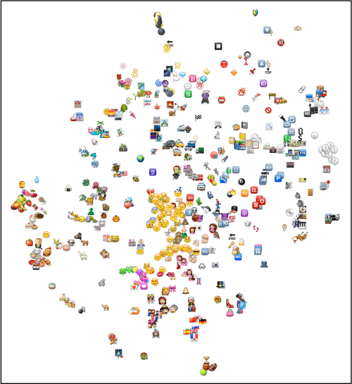
A hundred dimensions are pretty hard for humans to visualize. To visually inspect the relationships between emoji, we can take our 100-dimensional representation for emoji, reduce it two dimensions, and then plot them on a grid. We do this using an algorithm called t-SNE, which attempts to preserve relationships in a visually meaningful way:

Many clusters emerge: food emoji on the left, opposite the work emoji in the top right. Shoes (bottom right) are associated closely to handbags while bathing suits are closer to the water and marine animals (top left). Alcoholic drinks (bottom left) cluster together with bowling. Towards the center, we see a large clustering of facial expressions bordered by sadness, shock, laughter, happiness and coolness. As we travel downwards, we can see happy, love leading all the way the family and wedding emoji.

One has to be careful not to read *too* much into the representation since it is an attempt to produce a 2D space out of a 100D one. But it’s clear that semantics are being approximated in our representation.

Part-1-ing Thoughts

On Instagram, emoji are becoming a valid and near-universal method of expression in all languages. Emoji usage is shifting the people’s vocabulary on Instagram and becoming an important means of expression: their use is anti-correlated with internet slang like “lol” and “xoxo.” By observing words and emoji together we were able to discern representations of both. These representations can help us better understand their semantics and find distinctive characteristics of similar symbols.

Stay tuned for Part 2 on how we actually implemented emoji hashtags. #😳

Thomas Dimson is a Software Engineer on the Instagram Data Team, and also created Instagram’s Hyperlapse app.

Improving Comment Rendering on Android

instagram, android, performance, WWIM11,

Last weekend, thousands of Instagrammers from all over the world got together for Worldwide InstaMeet 11, one of Instagram’s community-organized, real-world meetups. #WWIM11 was our largest and most geographically diverse InstaMeet ever - thousands of Instagrammers from Muscat to Bushwick shared over 100k photos.

With over 300 million people around the world using Instagram every month, 65% of whom live outside the U.S., we’re always working to make Instagram faster and easier to use for people no matter where they are. And since our Android redesign last summer, we’ve continued to make performance improvements that allow us to scale better and faster.

One of our recent improvements was addressing the challenge of rendering long, complex text on Android and how to optimize it for Instagram’s feed scrolling. We hope you can use some of what we learned to make your own apps faster!

Product Requirements and Performance Issues

On Instagram, your feed is composed of beautiful photos, videos, and text. For every photo and video, we display the full caption and the five latest comments. Since people frequently like using captions to tell the story behind their photos, they are often long, complex, and may contain links and emojis.

The main issue with rendering such complex text is the performance hit it creates on scrolling. Text rendering in Android is slow. Even on a new device like the Nexus 5, the initial text drawing step for a complex caption with a dozen lines of text can take up to 50ms, and the text measuring step can take up to 30ms. All of these steps happen on the UI thread, and can cause the app to drop frames when the user is scrolling.

Here are a few tips that have helped us optimize comment text rendering for the Instagram Android app.

Use text.Layout, Cache text.Layout

Android has different widgets to display text on screen, but under the hood, they all use text.Layout to do rendering. For instance, the TextView widget will convert the String to a text.Layout object, and use canvas API to draw the text.Layout object on screen.

text.Layout object is inefficient to create since it measures the text’s height in its constructor. Caching and reusing text.Layout instances can save time. The TextView widget in Android doesn’t provide a set TextLayout method on the TextView, but it’s not hard to write one yourself.

Using a custom view to draw text.Layout manually also has performance advantages: TextView is a general-purpose widget which supports a lot of features. If we just needed to render static, clickable text on screen, things would be much simpler:

We could avoid unnecessary conversion from SpannableStringBuilder to String. Depending on whether your text has links in it, TextView under the hood may do a copy operation on your string, which would cause a lot of allocations.
We could always use StaticLayout, which is slightly faster than DynamicLayout.
We could avoid all unnecessary logic in TextView: the logic to watch changes in text, the logic to properly layout the embedded drawable, the logic to draw the editor, and the logic to pop up a drop-down list.

Using TextLayoutView, we can now cache and reuse the text.Layout, instead of spending 20ms every time when we call TextView#setText(CharSequence c).

Warm up the Layout Cache after We Download the Feed

Since we know we are going to show these comments after we download them, a simple improvement we made was warming up the cache after we download all of stories.

Warm up TextLayoutCache after You Stop Scrolling

After being able to cache the text.Layout, we get the constant measure time and binding time. But the initial drawing time is still relatively long. The 50ms drawing time results in noticeable jitters.

Most of these 50ms times were taken by measuring text advances and generating text glyphs. They are all CPU operations. To improve text rendering speed, Android introduced TextLayoutCache in ICS to cache these intermediate results. It is an LRU cache and cache keys are text lines. If you hit the cache, the text drawing speed would be much faster.

During our test, the cache could reduce the text drawing time from 30ms-50ms to 2ms-6ms.

To get good drawing performance, we can warm up this cache before we draw the text on screen. The idea is virtually drawing this text on an off-screen canvas. This way we can warm up the TextLayoutCache on a background thread before we draw the text on screen.

The size of TextLayoutCache is default to 0.5M, which is large enough to hold all comment text for a dozen photos. We decided to warm up the cache as soon as user stops scrolling, we look ahead and warm up five stories on the current scrolling direction. At anytime, we have at least five stories in cache on each direction.

After applying all these optimizations, the number of dropped frames was reduced by 60% and the total number of jitters was reduced by 50%. We hope you can apply some of these learnings to your own apps to improve speed and performance. Let us know what you think - we look forward to hearing about your experiences!

By Kang Zhang, Instagram Android engineer

Migrating from AWS to AWS

instagram, infrastructure, migration, aws,

In an earlier blog post, we gave a high level description of our migration from AWS to FB data centers. What follows is an in-depth analysis of how we migrated thousands of running AWS EC2 instances into Amazon’s Virtual Private Cloud (VPC) in the span of 3 weeks with no downtime. It was extremely meticulous work, and it required the development of custom virtual networking software to make it happen. It was, as far as we are aware, the fastest and one of the largest EC2 to VPC migrations to date.

Investigating Direct Connect

Direct Connect is a product offered by AWS that allows a customer to establish peering links between Amazon’s data centers and a third party. Using it, we figured that we could link to Facebook’s infrastructure over multiple redundant 10Gbps links. It was during this research when we found the main blocker:

We have no control over IP addressing in EC2.

While this hadn’t been an issue before, it was impassable if we were to establish links with Facebook, as their internal IP space intersected with that of EC2. After much deliberation, we began to understand that we had one option: migrate to VPC first.

VPC launched in mid 2009 as a companion product to the existing EC2 offering, though it quickly became considered to be EC2 2.0, as it remedied many of the commonly accepted EC2 downfalls. At face value, the migration didn’t seem conceptually difficult, as VPC was just another software abstraction on top of the same hardware, yet it was much more complex, with a few main issues:

You cannot migrate a running instance.
AWS offers no migration plan.
EC2 and VPC do not share security groups.

This last point lingered in our heads as we tried to come up with a solution. What would it take to make EC2 and VPC talk to each other as if the security groups could negotiate? It seemed insurmountable: we had thousands of running instances in EC2 and we could not take any downtime. We were looking for a solution that would allow us to migrate at our own pace, moving partial and full tiers as needed, with secure communication between both sides.

So, we created Neti, a dynamic iptables-based firewall manipulation daemon, written in Python, and backed by Zookeeper.

Design and Implementation of Neti

Neti is the name of the Sumerian gatekeeper to the Underworld. The name seemed fitting, as we needed an all-knowing gatekeeper that would control access to and from both EC2 and VPC. We had several requirements during the design process:

Security: Neti must keep unauthorized traffic off of our instances on both sides.
Abstraction: Neti must allow the instances on both sides to communicate seamlessly, without knowledge at the application layer about where each instance was located.
Automation: We have too many instances to curate access lists, so Neti must be fully aware of any instance changes in either network. It also must be deployable and upgradeable using configuration management software.
Performance: All of this must occur without any significant increases in latency.

Due to the lack of integration options between EC2 and VPC, the only route for communication is over the instances’ public interfaces. Using EC2 security groups, each group would need to be aware of the public IP of every instance with which it communicated. If we had tens of instances (or even hundreds), this might have been manageable. Yet, with thousands of instances on each side, trying to control the security group access lists would be unwieldy. Also, security groups in EC2 tend to negatively affect network performance as the number of rules increases.

So, we looked towards iptables to provide the security we needed. Iptables is the standard for Linux packet filtering, and can scale much better than EC2 security groups. Each instance has its own iptables firewall, and Neti manipulates the iptables rules as needed. Once the instances are locked down with iptables, the EC2 and VPC security groups get opened up to allow all traffic from any public AWS IP range.

Additionally, iptables helps to provide a mechanism for achieving our desired abstraction layer. Neti assigns each instance an “overlay” IP address which is used at the application layer for communication. This IP is configured as a DNAT record, pointing at the instance’s IP. This way, the application sees the same IP regardless of the instance’s location in EC2 or VPC.

All of this is coordinated by Zookeeper, which keeps all of the registration information about every running instances.

Architecture

There are three components to the system: the Neti daemon, a Zookeeper cluster, and a set of Zookeeper proxies.

Neti Daemon: The Neti software must be run on each instance.

Zookeeper Cluster: You must run a Zookeeper cluster within VPC, configured with its own security group.

Zookeeper Proxies: As we’ll need instances in both EC2 and VPC to communicate with Zookeeper, there must be EC2 instances set up in an identical arrangement to the VPC cluster, placed within their own security group, and set up to proxy all requests to the VPC cluster. This security group, as well as that of the VPC cluster, must allow all Zookeeper traffic between them on their public instances. For ease of instance replacement, it’s a good practice to attach Elastic IPs to these. These are the only instances that will not run Neti, as Neti relies on these clusters to operate.

Neti Instance Lifecycle

Let’s say we have three instances: Hudson, Sierra, and Walden. Hudson and Sierra live in EC2, and Walden has already been migrated to VPC.

As the Neti daemon starts on Hudson, it begins the registration:

Neti contacts Zookeeper1-proxy, and, using its instance ID, inquires if it has ever been registered. If found, it gets the same overlay IP as before. If not, it randomly chooses an available overlay IP and locks it to this instance ID.
Neti sends up the IP information and network location to Zookeeper to complete registration.
Neti downloads the current list of running instances from Zookeeper, including all of their public, private, and overlay IPs, as well as the network they live in.
The list is parsed, and iptables filter and DNAT rules are generated for each of the entries.
Neti sets a watch on the Zookeeper instance list.

Concurrently, as soon as step 2 finishes, all the rest of the registered instances get their Zookeeper watches triggered with the new set of instance data, and their iptables configs get updated automatically.

Once this dance is complete, all of the instances have full access to each other, and are successfully blocking any unauthorized traffic. If another instance spins up, this process starts again; if any instance dies, Zookeeper notifies all of the Neti daemons of the change and rules are updated within seconds across the entire fleet.

Overlay IPs and you

The overlay IP makes all instances agnostic to the location of the target instance. For example, let’s say that both Walden and Sierra are frontend instances and Hudson is a database server. Due to latency and security, you do not want Walden to communicate with Hudson over public IPs. Yet, you need Sierra to access Hudson over public IPs, as Hudson is still in EC2. With overlay IPs you do not have to build two different DB configs for each side, continuously updating and shipping the changes as you migrate servers to VPC. You simply use the overlay IP, and Neti handles choosing the optimal path.

Performance issues, or how I learned to stop restoring ip lists and love ipset

In v1 of the design, we were purely using iptables to manage all of the NAT and filter rules, leveraging the built-in iptables-save and iptables-restore tools. However, as we tested larger numbers of rules in iptables we started to hit performance issues. The problem occurs because every single request must do a O(n) lookup on the iptables filter to determine if it may proceed. Testing 8000 rules on one of our Memcached instances caused the network throughput to drop by an order of magnitude.

Clearly, we couldn’t continue if this was the case, so we looked elsewhere. After finding an article on iptables performance, we switched to using ipset for the implementation. It had a few major benefits:

It stored the list of IPs in a hash table in memory, offering O(1) membership checks
The set of IPs could be updated on the fly with simple command line tools.
It provided more peace of mind about the system, because we did not have to reload the entire iptables filter each and every time a host changed.

With ipset in place, we tested well over 8000 rules without any degradation of network throughput.

The Migration

For a migration like this, we knew that preparation was key. There were going to be parts of the system on either side of the “gap” at all times, with different timelines, strategies, and requirements for each tier. A quick stop/start forklift of the tiers would not work without downtime, so the entire migration had to be a finesse game, with the end-to-end process mapped out, analyzed, monitored, and executed.

Inventory

First, we had to take stock of everything. Everything. We spent a good deal of time cataloging every system in the fleet (remember spreadsheets?), along with their individual migration strategies and the potential problems that they may have. This effort had a three-pronged benefit:

We established confidence that each system could be migrated after planning out each step.
We constructed a high level view of our infrastructure and understood the weak points in terms of failover scenarios.
We found many systems that were either unnecessary or suitable for consolidation.

This migration (and the one to follow) allowed us to distill our infrastructure into a core set of critical systems, greatly easing migration and management going forward.

Tag all the things!

With the sheer number of instances we had to migrate, we relied on the instance-tagging feature of EC2. Most of our instance reporting and lookup tools were already built upon tags, tracking instance name, role, and some chef attributes, so adding some new metadata was simple. We used tags to track the installed Neti version, the overlay IP, and various Neti state information.

Tags also became useful in monitoring the process. We could run ad hoc reports to see how many instances have been migrated, how many were running old versions of Neti, and if any weren’t running Neti at all. We built some of these scripts into Sensu checks as well, so that we could be alerted to any issues. Having an arsenal of scripts to constantly watch the progress and status was essential to a smooth migration.

With Neti distributed throughout our infrastructure, we proceeded to flip on all access to public traffic into the AWS security groups. At this point, Neti controlled all access into these systems, and we could begin moving server tiers. Thanks to Neti, the entire infrastructure appeared to be operating on one large, flat network, simplifying the migration strategy.

Most tiers were migrated by bringing up identical tiers in VPC and cutting traffic over. For example:

Django: Our frontend tiers were stateless, so this was a simple matter of bringing up new hosts in VPC, and shutting down the old ones.
PostgreSQL: Using the streaming replication built into version 9.2, we were able to bring up master/slave replica sets in VPC, and cut to them with application-level controls. With this method, two of us cut over our entire DB fleet to VPC in less than 2 hours once the tiers were online and replicating.
Cassandra: The VPC hosts were brought online as members of another datacenter with respect to Cassandra configs, so replication and migration was simple.
Redis: New master/slave replica sets were synced to the current production slave (to avoid BGSAVE on the master) and the configs were cut over.

Hiccups

All in all, we had fewer issues than we had expected, especially considering this complex migration strategy. One problem was with conntrack. I can hear the groans already. Conntrack was a necessary evil in this scenario so that iptables did not need to be parsed on every connection. Here’s what happened: The instances did not have conntrack enabled, so when Neti was started, it built and loaded the iptables rules, which in turn enabled conntrack. On an instance with a lot of traffic, for example a Memcached instance, it takes a matter of seconds to overwhelm the default max of conntrack entries (65536). Then, new connections are denied, making the instance rather useless.

Mitigating this issue was rather simple. We forced chef to run a modprobe conntrack and set the nf_conntrack_max to a much higher limit before installing and starting Neti.

Conclusion

It took just less than 3 weeks to migrate everything to VPC. In the end, we built a large set of skills and guidelines that would help our next migration go just as smoothly. The main takeaways were:

Document everything. A well-documented infrastructure ensures that you will not forget any dependencies during the migration, and well thought out migration plans for each tier minimizes the roadblocks that you will hit. During the migration, you’ll be running in a heterogeneous environment, and you don’t want to get stuck there while you figure out the next steps.
Tooling can make or break a project. Investing time in Neti and expanding our tools to track the Neti rollout and audit the migration status were key to the migration being successful. Your tooling deserves love.
Don’t fear the low-level. Getting down and dirty with Iptables enabled this migration. This meant spending a lot of development time much closer to the kernel than normal, but this feat would not have been possible otherwise.

We have open sourced Neti and it’s companion Neti-cookbook for Chef. We hope that many people can benefit from our work on the problem and that it will ease their migration into VPC.

By Nick Shortway, Instagram infrastructure engineer

Building a better Instagram app for Android

instagram, instagram for android, android, instagram engineering, performance,

Android is a huge ecosystem, with more than 1 billion active users spanning thousands of different device models. People who use Android have an incredible amount of choice, with significant variations in speed, feature set, and cost. Screen size is the most obvious variable – popular Android devices span from 240 x 320 to 1080 x 1920 pixels, a 27-fold difference in pixel count! In some emerging markets, users must also contend with unreliable mobile networks. All this means that supporting Android users is both a technical challenge – and an opportunity for mobile developers who want to reach the entire world.

At Instagram we’ve spent the last year reimagining and redesigning our Android app to work better for our users, no matter what phones they use or where they are located. We shared details about this effort for the first time at this week’s @Scale conference.

We focused our work on Android on two key areas: design, and startup time.

Design

We redesigned Instagram for Android six months ago with three main goals in mind: making the app faster, more beautiful, and more screen-size aware.

“Flat design” has taken hold in the mobile world over the past few years. Android’s “Holo” theme, Windows Phone, and iOS7 all ditched complex gradients and shadows for solid colors and flat images. Flat design looks great on phone screens, but there is an even more important reason why it has taken hold: performance. Flat design is all about doing less — stripping away UI elements and letting the content speak for itself. Drawing solid colors on the screen is faster and more memory efficient than loading and displaying gradients from image files on disk. Simplicity means less work for the phone’s hardware, hence a faster app.

With these goals in mind, we rewrote every single screen in the app. We gave Instagram on Android a beautifully flat makeover, trimmed unnecessary UI to give you more space to view photos and videos, and focused relentlessly on doing less in order to make the app faster.

The most dramatic UI optimization happened in the photo- and video-capture and editing flow. We rewrote the original layout flow to be more screen-size aware. To do this we divided screens into four buckets, based on aspect ratio and DPI, and used a condensed layout on only the screens in the smallest buckets. At the same time, medium- and large-sized screens received an expanded layout that better utilized the available pixels. The result is that most Instagram’s Android users now experience a more ergonomically friendly flow, with all the editing and camera controls easily within reach of your thumb.

One of the techniques we use widely through the app is “asset tinting,” the ability to colorize assets programmatically. In a flat world, all of our assets are simply shapes, and we can change their colors at runtime. This allows us to eliminate separate assets for different UI states. Asset tinting is touted as a new feature in the upcoming Android L release, but it’s actually been possible in all versions of Android. You can apply a ColorFilter to a Drawable or an ImageView, and it will change the rendered output. We keep a static cache of immutable ColorFilter objects and reuse them all over the app.

In the end, we were able to dramatically reduce the number of assets needed display the Instagram UI when the app starts. We went from 29 assets to display the title bar and tab bar to 8. It turns out that not loading and decoding all those assets on startup gives you an awesome speed win; this alone reduced the app startup time by 120 milliseconds across devices (an improvement of roughly 10-20%, depending on the device). These gains were felt all across the app – for example, user profiles displayed up to twice as fast because of this simplification.

With this new flat design, and using the techniques described above, we were able to ship a smaller APK with fewer images. We cut the total number of assets in the app in half, even while adding xxhdpi assets. Along with other optimizations, the APK we shipped post-redesign was half the size of what it had been a few months before. This is a huge benefit for users who pay for data by the kilobyte and must wait for the app to download over really slow networks.

Startup Time

Users don’t want to wait forever for their apps to start up. This is especially important on Android, where less powerful phones will kill apps more often under memory pressure, making the impact of a long startup time even more painful.

We managed to cut the Instagram app start time in half over the past year on Android, to the point where it’s now one of the fastest-starting apps on the phone. Instagram now starts up and is usable in less than 0.5 seconds on a Galaxy S5, and in only 1.5 seconds on a Galaxy Y, an older device that has been popular in emerging markets.

To achieve these gains, we spent a lot of time profiling the app, both using the Android TraceView tool, and manual timing statements in the code. We made a lot of small improvements, like rewriting inefficient JSON parsing code and lazy-loading components that weren’t really needed for startup. There were two areas that required some creativity.

The first was in managing “heavy” app-wide singletons: services like our image cache, video cache, and http client. These need to be initialized for the app to work, right? Well actually, they don’t — we can start the app and interact with it without issuing network requests or showing any photos or videos. This means that these services can be lazy-loaded. However, we don’t want to complicate the programming model by having these objects be “null” during startup. So we initialize these objects in two steps. We create them on the main thread as we used to, but leave them in an uninitialized state, just enough so that the public API works. Then, when we spin up separate threads to actually load images or load content from the network, we finish initialization by doing the heavy lifting — loading SSL certificates off the disk, or opening and reading the cache journal file.

The second thing we found was that our News page was really slowing down app startup. The News page shows you who liked and commented on your photos, and we load it at startup so that you can see your new activity immediately. News was originally implemented as a webview, and after profiling we were surprised to find that it was creating a lot of threads on startup, stealing time from the main processor. We realized that we had no control over how the webview manages important system resources. It spins up its own networking stack, manages its own image cache – a lot of duplicated work with the rest of the app. To fix this, we converted News to be a native view. This gave us enough control to be able to delay loading News until after main feed is loaded, and to share the network stack and image cache with the rest of the app.

All of these efforts combined led to a much more usable Instagram for Android, which people have been enjoying for the past 6 months. Simplicity is a core principle for our engineering and product teams, and we’ll continue to push hard on efforts like these to make the Instagram experience as fast and beautiful as possible for all of our users.

By Tyler Kieft

Fast, auto-generated streaming JSON parsing for Android

Instagram, JSON parsing, Android, tech, performance,

The Instagram engineering team is constantly looking at how we can improve the speed, reliability and overall performance of the app. One of the things we wanted to improve is how quickly people using the Android app can view “News” in their Instagram feed—the place you go to see when people tag you, like or comment on one of your posts, or even to see what the people you follow are up to.

We started with Android after facing some special challenges on the platform converting data between formats. Large amounts of unstructured data needs to be parsed into meaningful constructs in an efficient manner. So, earlier this summer we developed a tool to automate this process, ig-json-parser, and today we’re happy to announce that we’re making it available to the open source community.

But first, a little background on why we’re doing this…

JSON is a prevalent data format for internet applications, and as such, serialization and deserialization to native objects on each platform is important. It is vital for these transformations to be correct, and desirable for them to be fast and efficient. On mobile platforms such as Android, there are additional challenges such as dalvik-specific issues and extreme memory pressure. Jackson ObjectMapper provides a mechanism which achieves most of these objectives, but comes up short in a few areas. First, ObjectMapper incurs a significant one-time penalty the first time it encounters an object it has not previously serialized/deserialized. This penalty is especially onerous when it affects the startup time of a mobile application. Second, ObjectMapper performs a lot of memory allocations, which can stress the garbage collector. Finally, it retains a large memory footprint even after the operations are complete.

Jackson stream parsing offers an alternative that solves all of the issues that ObjectMapper presents. Unfortunately, it introduces a fatal flaw of its own: stream parsing requires a lot of repetitive handwritten code, which is burdensome to write and prone to mistakes. Because of these issues, we have traditionally used them in limited areas where ObjectMapper can significantly degrade performance.

The ideal solution is to automatically generate the stream parsing code, which is what ig-json-parser does. It is a compile-time processor (known as a JSR-269 annotation processor) that takes model classes annotated with a few bits of data, and generates a stream parser. The mechanism is highly flexible, allowing users to plug in their own code snippets to customize the generated code.

The performance characteristics of the autogenerated parser are excellent. In the tables below, the test data is a list of Instagram stories.

On cold start, the benchmark yields:

On a subsequent iterations of parsing the data, the gap is significantly shorter:

At the end of the day, delivering the best possible experience for people is what’s most important to us and the ig-json-parser has helped us do just that. We’re excited about the opportunities the tool presents and looking forward to seeing how the community will use it within their own organizations.

Older Entries