Happy Anniversary α Centauri Bb?

by Paul Gilster on October 16, 2014

A physicist and writer well-versed in the intricacies of the exoplanet hunt, Andrew LePage now turns his attention to the question of planets around Centauri B, and in particular the controversy over whether the highly publicized Centauri Bb does in fact exist. Today is the second anniversary of the discovery announcement, and we still have work to do to resolve whether ‘noise’ in the data — explained below — may account for what seems to be a planet. The good news is that multiple teams continue to work on Alpha Centauri, and we should expect answers within several years, or just possibly, as LePage explains, a bit sooner than that.

by Andrew LePage

Andrew_LePage_2014

Time certainly seems to fly at times. It has already been two years since the October 16, 2012 announcement by a Geneva-based team of astronomers of the discovery of a planet orbiting our Sun-like neighbor, α Centauri B, using precision radial velocity measurements. While this planet, designated α Centauri Bb, was hardly the Earth-like planet for which interstellar travel enthusiasts had been waiting so long, its presence demonstrated that the closest star system to us harbored at least one planet and held the promise of more to be discovered. But two years after this momentous announcement, many questions still remain and this important discovery has yet to be independently confirmed.

First some background: at the heart of the α Centauri system 4.37 light years away are a pair of Sun-like stars, designated α Centauri A and B, locked in an eccentric 79.9-year orbit. The probable third member of this star system, located about 15,000 AU from the main pair of stars, is a dim red dwarf better known as Proxima Centauri. With a distance of 4.24 light years, it is the closest known star to our solar system. Despite the distance between α Centauri A and B varying from 11 to 35 AU during the course of one revolution, various dynamical studies performed over the decades have confirmed that regions with stable planetary orbits do exist in this system. These studies have shown that orbits out to about 3 AU, give or take, would be stable depending on their inclination to the plane of the orbit of α Centauri A and B about each other. What has not been so clear is if planets could form around this pair of stars.

A number of studies performed over the past couple of decades have been more or less evenly split on the question of whether or not planets could form around α Centauri A and B. Some studies have shown that the building blocks for planets, called planetesimals, would be able to collect themselves together into planets out to some reasonable distance. Still other studies have suggested that the presence of the two stars would have stirred up the orbits of the planetesimals too much. Instead of collecting into larger bodies, the planetesimals would tend to smash themselves apart upon contact so that planets could not form. As in the story about the ancient Greek philosophers arguing about how many teeth a horse has, it made sense to open the horse’s mouth and simply count them – it was time to look for planets orbiting α Centauri A and B.

Given the difficulty of detecting extrasolar planets even in a nearby star system like α Centauri, the first technology that offered reasonable chance of success was the precision measurement of changes in the stars’ radial velocity resulting from the small reflex motion of an orbiting planet. But after almost two decades of measurements with increasingly better instruments, the results of searches for planets orbiting α Centauri A and B published up to 2011 had found nothing. This null result combined with dynamical arguments only demonstrated that planets larger than Saturn or Jupiter did not orbit within about 2 AU of either α Centauri A or B. This still left a lot of possibilities including Earth-size planets orbiting comfortably inside the habitable zones of these stars but much more precise radial velocity measurements would be required to detect them.

Beginning around seven years ago, several teams employing various observing approaches are known to have started looking for lower-mass planets orbiting α Centauri A and B with instruments capable of making radial velocity measurements with uncertainties on the order of one meter per second – a factor of up to four more precise than in previously published results for the system. The first team to announce any results from their search was the European team using the HARPS (High Accuracy Radial Velocity Planetary Searcher) spectrometer on the 3.6-meter telescope at the European Southern Observatory in La Silla, Chile. They employed a new data processing technique to extract the 0.5 meter per second signal of α Centauri Bb out of 459 radial velocity measurements they obtained between February 2008 and July 2011. These radial velocity data had a measurement uncertainty of 0.8 meters per second and contained an estimated 1.5 meters per second of natural noise or “jitter” resulting from a range of activity on the surface of α Centauri B modulated by its 38-day period of rotation.

centauri_system

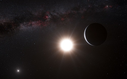
Image: An artist’s impression of the still unconfirmed α Centauri Bb whose discovery was announced on October 16, 2012. (Credit: ESO/L. Calçada/Nick Risinger)

The HARPS team’s analysis indicated the presence of a planet with a minimum mass or Mpsini (where i is the unknown inclination of the planet’s orbit to our line of sight) of just 1.1 times that of Earth, locked in a tight orbit with a radius of just 0.04 AU and a period of 3.24 days. This was well below the upper limits set by earlier searches. Given sufficient observation time, the team estimated that they could detect a planet with a Mpsini of about four times that of the Earth in a 200-day orbit inside the habitable zone of α Centauri B. While the result generated much excitement, it was also met with a healthy amount of skepticism in the astronomical community because of the previously untried technique used to process the data to extract such a low-amplitude signal.

One of the first critics, American astronomer Artie Hatzes (Thuringian State Observatory, Germany), performed his own analysis of the publicly available HARPS data set using two different data processing techniques to look for the radial velocity signal of α Centauri Bb. Formally published in June 2013, Dr. Hatzes’ analysis did indeed find a signal buried in the radial velocity data with a period of 3.24 days but it had a false alarm probability of a few percent – far too high to be considered a reliable detection. Furthermore, his analysis of the “random” noise in the data showed that it had periodicities in the 2.8 to 3.3 day range and amplitudes on the order of half that of the alleged planetary signal. Given the recent situation of planetary false alarms with GJ 581 and GJ 667C, this finding suggested that noise in the data, whether from the instrument or activity on α Centauri B, might have been mistaken for a planet. Dr. Hatzes concluded that additional data were needed to better understand the nature of the noise in the radial velocity measurements and confirm the planetary nature of the radial velocity signal.

Other teams have already been taking data in order to confirm the existence of α Centauri Bb as part of their ongoing observing programs although no results have been formally published to date. A team of astronomers working with the 1.5-meter telescope at Cerro Tololo Inter-American Observatory (CTIO) in Chile are using CHIRON (CTIO Higher Resolution Spectrometer) to search for planets orbiting α Centauri A and B in part with the support of The Planetary Society. The project’s principal investigator, Debra Fischer (Yale University), quoted in a blog on The Planetary Society’s web site posted earlier this year that they had insufficient data to detect α Centauri Bb when its discovery was announced in October 2012. They launched a renewed effort to gather much more data at a higher cadence starting in 2013 aimed specifically at detecting the purported planet’s 3.24-day signal. To date they have not detected α Centauri Bb in their data but their simulations indicate that any such detection would have been marginal at best so far.

One of the issues complicating continuing efforts to gather more data needed to resolve the situation with α Centauri Bb is the increasing amount of stray light from α Centauri A that is degrading the quality of radial velocity measurements. As viewed from the Earth, the apparent separation of α Centauri A and B has been decreasing at an accelerating rate for about a third of a century as they move in their inclined elliptical paths around each other. The two stars will reach a near-term minimum separation of just four arc seconds at the end of 2015. The conventional wisdom has been that it will be several more years before the separation of α Centauri A and B increases enough to acquire new data of sufficient quality to confirm α Centauri Bb. But we might not have to wait this long after all.

One of the other groups known to be searching the α Centauri system for planets is a team of astronomers using the HERCULES (High Efficiency and Resolution Canterbury University Large Echelle Spectrograph) spectrograph on the one-meter McLellan Telescope at the Mt. John University Observatory in New Zealand. In July 2014 they submitted a paper for publication where they described a new technique to reduce significantly the effects of stray light contamination in precision radial velocity measurements.

In order to test the effectiveness of their new technique, they observed four double-line spectroscopic binaries (i.e. pairs of unresolved stars that can only be differentiated by periodic Doppler shifts in their spectral lines) whose blended images represent the worse-case scenario of “contamination”. With the new technique, they were able to recover accurate radial velocities of both components of the observed spectroscopic binaries. The New Zealand-based team now plan to use their new analysis method to reduce the data they are continuing to gather as part of their observing campaign of α Centauri that started in 2007. Their calculations show that they should be able to detect α Centauri Bb if it exists. If they are successful, the situation with α Centauri Bb might be resolved much sooner than later.

A more detailed account with general references to the discovery of α Centauri Bb along with more background information on the system can be found on my web site in the post titled The Search for Planets Around Alpha Centauri. A second post in this series, The Search for Planets Around Alpha Centauri – II provides details of the results of past searches for planets orbiting α Centauri A and B as well as what current and soon-to-be-started search programs hope to find.

tzf_img_post

{ 8 comments }

A Sunset Glimpse of Deep Time

by Paul Gilster on October 14, 2014

A truncated schedule this week as I attend to a pressing project that needs all my attention. So no post today or Wednesday, but back Thursday with a look at the Alpha Centauri planet hunt and the still-unresolved question of Centauri Bb. For the short interval, I’ll leave you with this quote from Lee Billings on the nature of deep time and genuine perspective.

Deep time is something that even geologists and their generalist peers, the earth and planetary scientists, can never fully grow accustomed to. The sight of a fossilized form, perhaps the outline of a trilobite, a leaf, or a saurian footfall can still send a shiver through their bones, or excavate a trembling hollow in the chest that breath cannot fill. They can measure celestial motions and list Earth’s lithic annals, and they can map that arcane knowledge onto familiar scales, but the humblest do not pretend that minds summoned from and returned to dust in a century’s span can truly comprehend the solemn eons in their passage. Instead, they must in a way learn to stand outside of time, to become momentarily eternal. Their world acquires dual, overlapping dimensions— one ephemeral and obvious, the other enduring and hidden in plain view. A planet becomes a vast machine, or an organism, pursuing some impenetrable purpose through its continental collisions and volcanic outpourings. A man becomes a protein-sheathed splash of ocean raised from rock to breathe the sky, an eater of sun whose atoms were forged on an anvil of stars. Beholding the long evolutionary succession of Earthly empires that have come and gone, capped by a sliver of human existence that seems so easily shaved away, they perceive the breathtaking speed with which our species has stormed the world. Humanity’s ascent is a sudden explosion, kindled in some sapient spark of self-reflection, bursting forth from savannah and cave to blaze through the biosphere and scatter technological shrapnel across the planet, then the solar system, bound for parts unknown. From the giant leap of consciousness alongside some melting glacier, it proved only a small step to human footprints on the Moon. The modern era, luminous and fleeting, flashes like lightning above the dark, abyssal eons of the abiding Earth. Immersed in a culture unaware of its own transience, students of geologic time see all this and wonder whether the human race will somehow abide, too.

Lee Billings, from Five Billion Years of Solitude (2013), p. 145.

the-cliff-etretat-sunset_big

Image: The Cliff, Etretat, Sunset, by Claude Monet, a work that has always somehow transcended time for me and inspired thoughts on Billings’ ‘abiding Earth.’

tzf_img_post

{ 14 comments }

Mapping the Weather on WASP-43b

by Paul Gilster on October 13, 2014

On Friday I mentioned transmission spectroscopy, the technique of analyzing the light of a parent star as it is filtered through a planetary atmosphere. We’ve used it on various ‘hot Jupiters’ before now — think of the much studied planet HD 209458b, where water vapor, carbon dioxide and methane have been detected and fierce upper atmosphere winds revealed. And while we wait to see if the method can be applied to the interesting WASP-94 system, we can look at its uses in another hot Jupiter whose weather has now been mapped.

WASP-43b has twice Jupiter’s mass and a breathtaking 19-hour year. Scientists using the Hubble Space Telescope have used transmission spectroscopy to determine the abundance of water in the atmosphere at the terminator between night and day on this tidally locked world. The team also used so-called emission spectroscopy — in which much of the light of the parent star is subtracted — to measure water abundance and temperature at different points in its orbit. What emerges from combining the two is a map relating weather and longitude.

“We have been able to observe three complete rotations — three years for this distant planet — during a span of just four days,” explained Jacob Bean (University of Chicago), leader of the research project. “This was essential in allowing us to create the first full temperature map for an exoplanet and to probe its atmosphere to find out which elements it held and where.”

Exoplanet WASP-43b orbits its parent star

Image: In this artist’s illustration the Jupiter-sized planet WASP-43b orbits its parent star in one of the closest orbits ever measured for an exoplanet of its size — with a year lasting just 19 hours. The planet is tidally locked, meaning it keeps one hemisphere facing the star, just as the Moon keeps one face toward Earth. The color scale on the planet represents the temperature across its atmosphere. This is based on data from a recent study that mapped the temperature of WASP-43b in more detail than has been done for any other exoplanet. Credit: NASA, ESA, and Z. Levay (STScI).

As we might expect, a planet in this configuration is a place of violent weather. The researchers find high-speed winds moving from the day side, where the temperature is above 1500 degrees Celsius, to the night side, where temperatures are in the 500 degree Celsius range. The two-dimensional maps of the planet’s atmospheric temperatures help us define the circulation patterns that show this heat transport under conditions of tidal lock.

We learn that WASP-43b is hot enough that all the water in its atmosphere is vaporized rather than producing extensive cloud cover — in fact, the planet reflects little of the parent star’s light. Water vapor is a useful tool. We know all too little of the water abundances in the gas giants of the outer Solar System because water is found deep inside their atmospheres in the form of ice. A hot Jupiter like WASP-43b opens the door for direct study of water in the form of vapor. The measurement is important because of the role water ice is thought to play in the standard core accretion model of gas giant formation, where solid particles collide, merge and grow into gradually larger bodies until a planetary embryo emerges.

Ahead for the water-mapping team is to make similar measurements for the atmospheres of other planets to study their chemical abundances. The paper on the water-mapping study explains why data from a wide variety of planets should help as we move into the era of the James Webb Space Telescope and other increasingly sensitive instruments:

…a planet’s chemical composition depends on many factors, including the planet’s formation location within the protoplanetary disk, the composition, size and accretion rate of planetesimals, and the planet’s migration history. Even perfect constraints on the abundances of many chemical species for a small number of objects may not yield a unique model for the origin of giant planets. Fortunately, the plethora of transiting exoplanets that have already been found and will be discovered with future missions offer the potential for statistical studies. Measuring precise chemical abundances for a large and diverse sample of these objects would facilitate the development of a more comprehensive theory of planet formation.

The day will come when we’re performing the same kind of measurements on Earth-sized worlds around other stars, something to keep in mind as we move into the JWST era.

Two papers present the WASP-43b work. The first is Stevenson et al., “Thermal structure of an exoplanet atmosphere from phase-resolved emission spectroscopy,” published online in Science 9 October 2014 (abstract). The water mapping study is Kreidberg et al., “A Precise Water Abundance Measurement for the Hot Jupiter WASP-43b,” accepted at Astrophysical Journal Letters (preprint). This time-lapse video shows the profile of WASP-43 over the course of a single planet rotation. A Hubble news release is available.

tzf_img_post

{ 2 comments }

A Planet Each for Stars in Binary System

by Paul Gilster on October 10, 2014

The WASP Consortium (Wide Angle Search for Planets) has come up with an interesting find: Two new Jupiter-class worlds, one around each star in a binary star system. Both are ‘hot Jupiters,’ a class of planets that is susceptible to discovery by transit methods, as in this case, and radial velocity as well. Consisting of two robotic observatories, one on La Palma (Canary Islands) and the other in South Africa, WASP has a proven track record, having found over 100 planets since 2006. WASP-94A and WASP-94B, like all WASP candidates, were confirmed by radial velocity techniques through a collaboration with the Geneva Observatory.

The two stars are about 600 light years away in the constellation Microscopium. In this case, it was the WASP-South survey team that noticed dips in the light of WASP-94A, the mark of a likely hot Jupiter, with WASP-94B being found by the Geneva team during the confirmation process for the first planet. “We observed the other star by accident, and then found a planet around that one also!”, says Marion Neveu-VanMalle (Geneva Observatory), lead author of the paper on this work.

wasp_transit_small

Image: A WASP planet transiting its host star. Credit: Mark Garlick.

We’ve sometimes speculated in these pages about a close binary system like Centauri A and B, wondering whether there could be planets around each star, a matter that remains undecided. WASP-94A and WASP-94B are in a much different situation — the estimated separation between the two is 2700 AU. The paper lists three other binary systems with pairs of planets. Like WASP-94, HD20782/HD20781 is a wide binary, with HD20782 hosting a Jupiter-mass planet and HD20781 two Neptune-class worlds.

We also have Kepler-132, an interesting system hosting three ‘super-Earths,’ with an angular separation too small to allow us to tell which of the two stars the planets are transiting, although researchers believe that the two planets with the shortest periods cannot be orbiting the same star. Finally, there is XO-2, another wide binary in which one star hosts a transiting hot Jupiter, while the other hosts two gas giants, one Jupiter-class, the other the mass of Saturn.

We may learn something interesting about the formation of hot Jupiters from the WASP-94 system. Planets like these should form far enough from their primary to allow ices to freeze out of the protoplanetary disk, while being later forced, presumably through interactions with another star or planet, into the inner system. The paper comments: “The discovery of a hot Jupiter around each star suggests that the same formation process took place and that similar favorable conditions boosted the migration of the planets.” Interactions between the two stars are problematic given the large separation but this may help us stretch our theories:

Even though at this stage nothing can be proven, there are recent dynamical theories relevant to this system. Moeckel & Veras (2012) described interactions in which a planet orbiting one component of a stellar binary can ‘jump’ to the other star. If the two giant planets were formed around the same star, planet-planet scattering could have occurred. This would have pushed one of the planets near the host star and ejected the second one, which could then have been captured by the stellar companion. As we do not know the eccentricity of the stellar system, we can also consider the ‘flipping machanism’ described by Li et al. (2014), in which a coplanar system leads to very high eccentricities for the planet.

We may also find the WASP-94 system valuable on other grounds. Like most of the WASP planets, WASP-94A and WASP-94B orbit stars that are relatively bright — most of the Kepler stars, by contrast, are faint. This Keele University news release quotes the university’s Coel Hellier speculating on the possibility of atmospheric studies through transmission spectroscopy, where the atmosphere of the transiting world can be analyzed as it moves onto and off the stellar disk during a transit. I can scarcely imagine what John Herschel, who first observed this stellar system back in 1834, would have made of possibilities like these.

The paper is Neveu-VanMalle et al., “WASP-94 A and B planets: hot-Jupiter cousins in a twin-star system,” in press at Astronomy & Astrophysics (preprint).

tzf_img_post

{ 14 comments }

The Emergence of Solitary Stars

by Paul Gilster on October 9, 2014

Looking at the latest work from Carnegie’s Alan Boss reminds me once again of the crucial role computers play in astrophysical calculations. We’re so used to the process that we’ve come to take it for granted, but imagine where we’d be without the ability to model complex gravitational systems. To understand planet formation, we can simulate a protoplanetary disk around a young star and let a billion years pass in front of our eyes. And as our models improve, we can set the process in motion with ever greater fidelity.

Read Caleb Scharf’s The Copernicus Complex ( Farrar, Straus and Giroux, 2014) to see how much we’ve learned by ever more precise modeling. Back in the late 1980s, Jacques Laskar (Bureau des Longitudes, Paris), Gerald Sussman and Jack Wisdom (the latter two at MIT) developed mathematical approaches that could track changes to orbital motions to understand our solar system’s past. Their work and the wave of innovation that followed helped us understand exponential divergence over million-year time periods, a crucial factor, as Scharf shows, in how unpredictable planetary motions can be:

Newton’s physics and its application by scientists like Laplace had appeared to be describing a clockwork universe, a reality based on laws that could always lead you from point A to point B, through space and time. And although the concepts of chaos and nonlinearity were well-known by the time these numerical computer experiments were carried out on planetary motions, this was the first real confirmation that our solar system was neither clockwork nor predictable.

In other words, when dealing with astronomical time-frames, we begin to find outcomes that could not have been predicted as we run our simulations. We’re observing chaos at play in complex gravitational systems, where tiny interactions can ultimately change the trajectories of entire planets. Scharf’s discussion of these matters celebrates the computer’s ability to model these phenomena and observe different results, but it’s also a humbling reminder of our limitations in thinking that with enough information we can always predict the outcome.

Learning How Stars Form

What Alan Boss is modeling is the formation of stars, using three-dimensional models of the collapse of magnetic molecular cloud cores. His simulations depict the formation of stars as clusters of newly formed protostars come apart. What they show is that younger star and protostar populations have a higher frequency of multiple-star systems than older ones. In other words, many single-star systems like our own start out as multi-star systems, with stars being ultimately ejected to achieve stability. You can see the modeling at work below.

boss_79864_web

Image: The distribution of density in the central plane of a three-dimensional model of a molecular cloud core from which stars are born. The model computes the cloud’s evolution over the free-fall timescale, which is how long it would take an object to collapse under its own gravity without any opposing forces interfering. The free-fall time is a common metric for measuring the timescale of astrophysical processes. In a) the free-fall time is 0.0, meaning this is the initial configuration of the cloud, and moving on the model shows the cloud core in various stages of collapse: b) a free-fall time of 1.40 or 66,080 years; c) a free-fall time of 1.51 or 71,272 years; and d) a free-fall time of 1.68 or 79,296 years. Collapse takes somewhat longer than a free-fall time in this model because of the presence of magnetic fields, which slow the collapse process, but are not strong enough to prevent the cloud from fragmenting into a multiple protostar system (d). For context, the region shown in a) and b) is about 0.21 light years (or 2.0 x 10¹⁷ centimeters) across, while the region shown in c) and d) is about 0.02 light years (or 2.0 x 1016 cm) across. Credit: Alan Boss.

As the molecular cloud that will form a star collapses, how it fragments depends, Boss shows, on the initial strength of the magnetic field. If the magnetic field is strong enough, single protostars emerge, but below this level, the cloud begins to fragment into multiple protostars. From the paper:

The calculations produce clumps with masses in the range of ~0.01 to 0.5 M, clumps which will continue to accrete mass and interact gravitationally with each other. It can be expected that the multiple systems will undergo dramatic subsequent orbital evolution, through a combination of mergers and ejections following close encounters, resulting ultimately in a small cluster of stable hierarchical multiple protostars, binary systems, and single protostars. Such evolution appears to be necessary in order [to] produce the binary and multiple star statistics that hold for the solar-type stars in the solar neighborhood…

Those statistics are striking. Roughly two-thirds of the stars within 81 light years of the Earth are either binary or part of multi-star systems. And because what we see today as single stars can also be the result of ejection from a multi-star system, the formation of binary and multi-star systems seems to be commonplace. I’m interested in these findings because if we are to understand our own place in the cosmos, we’re beginning to see that we have to account for why single-star systems do not seem to be the default in the Milky Way.

The paper is Boss and Keiser, “Collapse and Fragmentation of Magnetic Molecular Cloud Cores with the Enzo AMR MHD Code. II. Prolate and Oblate Cores,” in press at The Astrophysical Journal (preprint).

tzf_img_post

{ 5 comments }

Interstellar Flight: Risks and Assumptions

by Paul Gilster on October 8, 2014

The interstellar mission that Dana Andrews describes in his recent paper — discussed here over the past two posts — intrigues me because I’m often asked what the first possible interstellar mission might be. Sure, we can launch a flyby Voyager-class probe to Alpha Centauri if we’re willing to tolerate seventy-five thousand years in cruise, but what would we accept by way of acceptable cruise times? The lifetime of a human being? Multiple generations? And if we had to launch as soon as possible, what would the mission parameters be?

The mission that Andrews conceives grows out of questions like these. I can say upfront that this isn’t a mission I would want to fly on. For one thing, it’s a generation ship, so entire lives will be spent in cramped quarters, and the prospect of being overtaken by a later, faster ship is always there. But that’s not the point. 18th Century voyagers with a yen for the unknown could have waited for the age of steamships, but how could they have anticipated it? In any case, waiting would have cost them the journey that was in front of them. I think there will always be pioneers in search of experience unique to them, the first to step onboard as long as a viable mission presents itself.

Yesterday we looked at various propulsion strategies for Andrews’ starship, including a personal favorite, the Sailbeam design of Jordin Kare, which uses tiny micro-sails driven by laser as a stream of beamed energy that can be ionized when it arrives at the ship, providing thrust to a magsail. Dana Andrews knows a lot about magsails — working with Robert Zubrin in 1988, he showed that Robert Bussard’s interstellar ramjets would produce more drag than thrust, and the idea of turning a magnetic scoop into a magnetic sail began to grow. We’re seeing that it can be used both for acceleration and deceleration upon arrival.

Andrews_magsail

Image: Interstellar generation ship configured for braking. Credit: Dana Andrews.

Several decades before the Andrews/Zubrin paper, Robert Forward had been taking note of laser developments at Hughes Research Laboratories in Malibu, CA. He already knew about solar sails, which had appeared in the work of Konstantin Tsiolkovsky and Fridrikh Tsander in the 1920s and which had been the subject of a technical paper by Richard Garwin in 1958. As a science fiction writer, Forward was surely aware as well of Carl Wiley’s “Clipper Ships of Space” article, which appeared under the byline Russell Saunders in Astounding Science Fiction. Why not, Forward mused, boost a solar sail with a laser?

I can see why Andrews included Forward’s laser lightsail ideas in the current paper, but the magsail seems like a far more likely candidate for the near-term mission that he describes. Even working with a minimal Forward configuration, we still have to solve problems of deployment and infrastructure that are huge, including, in Andrews’ calculations, a beam aperture fully 20 kilometers in diameter. He goes on to describe a lightsail mission with acceleration of 0.05 gees that reaches 2 percent of c in 155 days at a distance of 267 AU. “The minimum cost system is to invest in really good stationary optics,” he adds, “thereby allowing less power and smaller sails, but then beam jitter begins to dominate.”

Summing up the various propulsion methods discussed, Andrews comments:

We quickly examined four different near-term interstellar propulsion concepts. Each has its issues… The laser-powered ion thruster needs aggressive weights for the design to close, but has no obvious showstoppers. The Neutral Particle Beam concept appears workable at planetary distances, but requires very high acceleration and power levels to maintain divergence angles of one microradian or more. Projecting a beam of neutralized particles presents the problem of re-ionizing a dispersed cloud of particles, which is a definite showstopper. The Sailbeam propulsion has potential, but needs tests of the acceleration capability and is still power hungry (~4000 TW of electrical power for the example presented here). Even at 4000 TW it needs pointing accuracy better than a nanoradian to finish the acceleration. The laser-lightsail actually came off as relatively low risk at 800 TW of electrical power, but that is very dependent on the availability of a 20 km diameter diffraction-limited steering optic, and a one-gram/m2 lightsail (both risk factor 4+).

Andrews_power

Image: Total energy usage comparison. Credit: Dana Andrews.

What makes predictions about spaceflight so tricky is that we can’t anticipate the emergence of disruptive technologies. The risk factors that Andrews develops as he looks at the progress of interstellar flight are, by his admission, estimates and ‘guesstimates,’ which is about the best we can do, and he characterizes near-term technologies as less than risk factor 4.

Andrews_risk

Image: Relative risk between candidate interstellar technologies.

We can all find things we might take exception to here and there in this list. You can see, for example, that Andrews characterizes a breakeven fusion reactor at risk factor 4, with a 40 year development time. Fusion has wreaked havoc with our predictions since the 1950s, and I think it’s optimistic to hope for working fusion power-plants even within this timeframe, though I know fusion-minded people who think we’re much closer. Fusion for starship propulsion he ranks at a risk factor of 7, needing 100 years to develop. Notice, too, that for the purposes of this mission, freezing or suspended animation are ruled out as being at risk factor 9, which would place their development 400 years out. A disruptive advance could negate this.

I find it useful to lay out our assumptions in such direct form. The biggest question I have regards fully closed-cycle biological ECLSS (Environmental Control and Life Support Systems). At a risk factor of 2.5 and 25 years of development, we could deploy these technologies on a generation ship, but will they be tested and ready by late in this century, when the starship would presumably be launched? My own guesstimate would lean toward a higher risk factor and 50 years for development, a tight but perhaps possible fit.

Other things the ship will need: Protection against galactic cosmic radiation (GCR), which Andrews proposes may be resolved by using magnetic fields to deflect charged particles away from the crew areas. He gives the topic a fuller discussion in a 2004 paper (see citation below). Dust in the interstellar medium poses a challenge because at 2 percent of c, impacting particles become plasma and can cause erosion to the spacecraft. Andrews notes this will need to be addressed in any starship design but doesn’t elaborate.

The conclusions [Andrews adds] are that near-term interstellar colonization flights are not completely science fiction, but there has to be a powerful requirement to generate the funding necessary to work many of the problems identified. The alternative is to wait a hundred years or so for low specific power fusion, or much longer for warp drive. We’ll see.

The paper is Andrews, “Defining a Near-Term Interstellar Colony Ship,” presented at the IAC’s Toronto meeting and now being submitted to Acta Astronautica. The 2004 paper is Andrews, “Things To Do While Coasting Through Interstellar Space,” AIAA-2004-3706, 40th AIAA/ASME/SAE/ASEE Joint Propulsion Conference and Exhibit, Fort Lauderdale, Florida, July 11-14, 2004.

tzf_img_post

{ 30 comments }

Pondering Interstellar Propulsion Strategies

by Paul Gilster on October 7, 2014

destination-moon-movie-poster-1950-1020142823

Back in 1950, George Pal produced Destination Moon, a movie that was based (extremely loosely) on Robert Heinlein’s Rocketship Galileo. Under the direction of Irving Pichel, the film explained the basics of a journey to the Moon — using among other things an animated science lesson — to a world becoming intrigued with space travel. I’ve wondered in the past whether we might one day have an interstellar equivalent of this film, a look at ways of mounting a star mission in keeping with the laws of classical mechanics. Call it Destination Alpha Centauri or some such and let’s see what we get.

Christopher Nolan’s film Interstellar doesn’t seem to be that movie, at least based on everything I’ve seen about it so far. I did think the early trailers were interesting, evoking the human urge to overcome enormous obstacles and buzzing with a kind of Apollo-era triumphalism. The most recent trailer looks like starflight is again reduced to magic, although maybe there will be some attempt to explain how what seems to be wormhole transit works. While we wait to find out, I still wonder about what kind of mission we would mount if we really did have a world-ending scenario on our hands that demanded an interstellar trip soon.

[Addendum]: I’ve been reminded that Kip Thorne has a hand in the science of this film, which does make me more interested in seeing it.]

Dana Andrews, as we saw yesterday, has been exploring a near-term interstellar colony ship that could fit into this scenario. Today I want to return to the paper he presented at the recent International Astronautical Congress. Andrews defines near-term this way:

Near-term means we can’t use warp drive, fusion engines, or multi-hundred terawatt lasers (which could destroy civilization on Earth in the wrong hands). Affordable means we’re going to do design and cost trades and select the lowest risk option with reasonable costs…. The goal was to design the system with state of the art technologies, assuming there will be twenty to thirty years of Research and Development before we start construction.

I speculated yesterday that given the need for a robust space-based infrastructure, it was hard to see the methods Andrews studies being turned to the construction of an actual starship before at least 2070, but it’s probably best to leave chronologies out of the picture since every year further out makes prediction that much more likely to be wrong.

The ‘straw man point of departure’ design in Andrews’ paper invoked beamed lasers mounted on an asteroid for risk stabilization and momentum control, with a 500 meter Fresnel lens directing the beam to the spacecraft’s laser reflectors, where it is focused on solar panels to power up ion thrusters using hydrogen propellant. A 32-day boost period gets the mission underway and a magsail is used to slow from 2 percent of c upon arrival. Andrews is assuming a laser output of around 100 TW to make this system work.

Enter the Sailbeam

But the point-of-departure method is only one possibility Andrews addresses. He also looks at Jordin Kare’s Sailbeam concept, in which a large laser array (250 5.8 TW lasers) accelerates, one after another, a vast number of 20 centimeter spinning microsails. The acceleration is a blinding 30 million gees over a period of 244 milliseconds, with the ‘beam’ being kept tight during the brief acceleration by using ‘fast acting off axis lasers,’ and additional lasers downrange. Only for the first 977 kilometers are the sails actually under the beam.

Andrews_sailbeam

Image: The Sailbeam propulsion schematic. Credit: Dana Andrews.

Notice the requirement for keeping the beam tight, an issue that has bedeviled concepts from laser-pushed lightsails to particle beam acceleration. After all, beam spread means you can’t deliver the bulk of the required power to the vessel that needs its energies. Assuming a tight microsail beam, however, the huge boost delivered at the beginning is sufficient, according to Kare’s numbers, to produce serious thrust for the starship. The beam reaches the ship, which vaporizes and ionizes the incoming sails by its own laser system, creating a plasma pulse that drives a magsail. Numerous issues arise with this method, as Andrews describes:

250 micro sails per second amounts to 3.2 kg/sec, and that requires 150 to 300 MW of laser power to ionize the microsails. Assuming 50% efficient lasers we need about a gigawatt of thermal power. Assuming risk factor three, that’s about 1000 mT of powerplant mass, which is actually less than the laser-powered ion propulsion system.

Could we beam the needed power to the ship? Perhaps, but there are other problems:

To maintain 0.01 gee with 250 microsails/second as the spacecraft approaches 2% c, we need to accelerate each microsail for 0.18 seconds. Since we assume each microsail launcher needs about 0.5 seconds to place, align, and spin up its microsail, we don’t need to increase the number of laser launchers to maintain the 0.01 gee. The problem is the long (730 day) acceleration time, which results in end of boost at 1238 AU. This requires very small sailbeam divergence (< Nano radian).

Andrews_microsail_interaction

Image: Microsail plasma interaction magsail dipole field. Credit: Dana Andrews.

With regard to the divergence problem, you’ll remember our recent discussions about neutral particle beams, which occurred in the context of Alan Mole’s paper in JBIS on a small interstellar probe. Mole, in turn, had drawn on earlier work by Andrews in 1994. In that paper, Andrews described a 2000 kilogram probe driven by a neutral particle beam sent to a magsail (the same magsail would be used for deceleration in the destination system). Writing in these pages, James Benford later found this propulsion method inapplicable for interstellar uses because of unavoidable spread of the beam and a corresponding loss of efficiency, although he considered it quite interesting as a driver for fast interplanetary travel.

In the current paper, Andrews revisits particle beam propulsion as a third alternative to the ion thrusters in his point-of-departure design. He cites Benford’s critique in the footnotes and goes on to add that the divergence of the beam will limit the useful range of operation. That implies high accelerations at the beginning of the flight, when the spacecraft can exploit maximum power from the beam as it meets the required divergence angle requirements. To catch up on our Centauri Dreams discussions of these issues, start with The Probe and the Particle Beam and Sails Driven by Diverging Neutral Particle Beams, both of which launched discussions and follow-up articles that can be found in the archives.

But there is a final possibility, the laser-driven lightsail as envisioned by Robert Forward back in the 1960s and refined by him in numerous papers in the years following. Which of these best fits our need to launch a near-term mission aboard a crewed starship? More on the laser lightsail and Andrews’ thoughts on energy requirements when I wrap up the paper tomorrow.

The paper is Andrews, “Defining a Near-Term Interstellar Colony Ship,” presented at IAC 2014 (Toronto) and in preparation for submission to Acta Astronautica. The earlier Andrews paper is “Cost considerations for interstellar missions,” Acta Astronautica 34, pp. 357-365,1994. Alan Mole’s paper is “One Kilogram Interstellar Colony Mission,” Journal of the British Interplanetary Society Vol. 66, No. 12, 381-387 (available in its original issue through JBIS).

tzf_img_post

{ 34 comments }

Starflight: Near-Term Prospects

by Paul Gilster on October 6, 2014

If our exoplanet hunters eventually discover an Earth-class planet in the habitable zone of its star — a world, moreover, with interesting biosignatures — interest in sending a robotic probe and perhaps a human follow-up mission would be intense. In fact, I’m always surprised to get press questions whenever an interesting exoplanet is found, asking what it would take to get there. The interest is gratifying but I always find myself having to describe just how tough a challenge a robotic interstellar mission would be, much less a crewed one.

But we should keep thinking along these lines because the odds are that exoplanetary science may well uncover a truly Earth-like world long before we are in any position to make the journey. I would expect public fascination with such a discovery to be strong. Dana Andrews (Andrews Space, now retired) has been pondering these matters and recently forwarded a paper he presented at the International Astronautical Congress meeting in Toronto in early October. It’s an intriguing survey of what could be done in the near-term.

How we define ‘near-term’ is of course the key here. Is fusion near-term or not? Let’s think about this in context of the mission Andrews proposes. He’s looking at a minimum transit speed of 2 percent of the speed of light (fifty years per light year), making for transit times in the neighborhood of hundreds of years, depending on destination. A key requirement is the ability to decelerate and rendezvous with the destination planet using a magnetic sail (magsail) that can be built using high-temperature superconductors. Andrews also assumes 20-30 years of research and development before construction actually begins.

The R&D alone takes us out to, say, 2040, but there are other factors we have to look at. As Andrews also notes, we have to assume that a space-based infrastructure sufficient to begin active asteroid mining will be in place, for it would be needed to build any of the systems we can imagine to make a starship. He cites a thirty-five year timeframe for getting these needed systems operational. Some of the R&D could presumably be underway even as this infrastructure is being built, but we also have to take into account what we know about the destination. Remember, it’s the Earth-like world discovery that sets all this in motion.

The ability to detect not just biosignatures but data of the kind needed for a human mission to an Earth-class planet may take twenty years or more to develop, and I think even that is a highly conservative estimate. For naturally we’re not going to launch a mission unless we have not just a hint of a biosignature but solid data about the world to which we are committing the mission. That might mean instruments like a starshade and perhaps interferometric techniques by a flotilla of observatories to pull up information about the planet’s surface, its continents and seas, and its compatibility to Earth-like life.

I’d say that backs us off at least to the mid-2030’s just for the beginning of exoplanet analysis of the destination, after which the planet is declared suitable and mission planning can begin. What technologies, then, might be available to us to begin interstellar R&D for a specific starship mission in, say, 2045, when we may conceivably have such detailed data, aiming at a 2070 departure if all goes well? Andrews doubts that high specific impulse, low power density fusion rockets will be available within the century, if then, and thinks that antimatter, if it ever becomes viable for interstellar propulsion, will follow fusion. That leaves us with a number of interesting alternatives that the paper goes on to analyze.

An Interstellar Point of Departure

Andrews develops an interesting take on using space-based lasers, working in combination with four-grid ion thrusters using hydrogen propellant and optimized for a boost period of thirty-two days. The specific impulse is 316,000 seconds. The lasers are mounted on a small asteroid (one or two kilometers) and take advantage of a 500-meter Fresnel lens that directs their beam to a laser reflector on the spacecraft. Let me take this directly out of the paper:

An actively steered 500 m diameter Fresnel lens (risk scale 3) directs the beam to the laser reflector on the Generation Ship Spacecraft, where it is focused onto hydrogen-cooled solar panels (risk factor 1), using a light-pressure supported ¼ wave Silicon Carbide reflector (risk factor 2.5). The light conversion panels operate at thousands of volts at multiple suns (risk factor 2) to allow direct-drive of four-grid Ion thrusters using hydrogen propellant and optimized for short life (30 days) and very low weight (risk factor 3). The four-grid thrusters provide a Specific Impulse (Isp) of 316,000 seconds operating at 50,000 volts using hydrogen. The triple point liquid hydrogen propellant is stored in the habitat torus during boost (the crew rides in the landing pods for the duration of the 32 day boost period), so there is no mass for propellant tanks. After acceleration the crew warms up the insulated torus, fills it with air, and moves in.

Andrews_Figure1

Image: The ‘point of departure’ design with associated infrastructure. Credit: Dana Andrews.

The ‘risk factors’ mentioned above refer to a ranking of relative risk for the development of various technologies that Andrews introduces early in the paper. Low Earth Orbit tourism, for example, ranks as a risk factor of 1, with development time in 10 years. Faster than light transport ranks as a risk factor 10, with development time (if ever) of over 1000 years. Low risk factor elements within the needed time-frame include asteroid-based mining and possible colonies, gigawatt-level beamed power, thorium fluoride nuclear space power and — this is critical for everything that follows — fully closed-cycle biological life support systems.

Andrews_Figure2

Image: Candidate generation ship configuration. Credit: Dana Andrews.

The habitation torus is assumed to be 312 meters in radius, rotating at two revolutions per minute to provide artificial gravity for the crew. The paper assumes a crew of 250, selected to provide differing skillsets and large enough to prevent problems of inbreeding — remember, we’re talking about a generation ship. The craft uses two thorium fluoride liquid reactors to provide power, acting as breeder reactors to reprocess fuel during the mission. Andrews comments:

The challenge to the spacecraft designer is to include everything needed within the 4000 mT allocated for end of thrust… This design closes but there is very little margin. For instance, there is only 15% replacement air and only 200 kg of survival equipment per person. All generation ships here use the same basic habitat and power systems.

Andrews_Chart

Image: Laser-powered ion propulsion generation ship description. Credit: Dana Andrews.

The magsail needed for deceleration takes, by Andrews’ calculations, 73 years to slow from 2 percent of c, with deployment at approximately 17000 AU from a star like the Sun, with the goal of entering orbit around the star at 3 AU, after which time the magsail can be used to maneuver within the system. Electric sails seem to work for operating inside the stellar wind, but Andrews notes that their mass scales linearly with drag, whereas a magsail’s mass scales as the square root of the drag desired. The magsail is thus the lighter option for this mission, envisioned here as a 6000 kilometer sail using high temperature superconductors, a technology the author believes will fit the proposed chronology.

The propulsion methods outlined here are what Andrews calls a “straw man point of departure (PoD) design,” with other near-term propulsion possibilities enumerated. Tomorrow I’ll take a look at these alternatives, all of them relatively low on the paper’s risk scale. The paper is Andrews, “Defining a Near-Term Interstellar Colony Ship,” presented at the IAC’s Toronto meeting and now being submitted to Acta Astronautica.

tzf_img_post

{ 66 comments }

Centauri Dreams welcomes Ravi Kopparapu, a research associate in the Department of Geosciences at Pennsylvania State University. He obtained his Ph.D in Physics from Louisiana State University, working with the LIGO (Laser Interferometer Gravitational-wave Observatory) collaboration. After a brief stint as a LIGO postdoc at Penn State, Ravi switched to the exoplanet field and started working with Prof. James Kasting. His current research work includes estimating habitable zones around different kinds of stars, calculating the occurrence of exoplanets using the data from NASA’s Kepler space telescope, and understanding the bio-signatures that can potentially be detected by future space telescope missions. Dr. Kopparapu’s website is http://www3.geosc.psu.edu/~ruk15/index.shtml.

by Ravi Kopparapu

Kopparapu_Photo

Imagine this scenario: You are planning to buy a new house in a nice neighborhood. The schools in the area are good, the neighborhood is very safe, but you want to know the ‘kid friendly’ area (so that your kids can have friends). You drive around, looking at the available houses, watching for any ‘kid signatures’. You notice that a good proportion of the homes in your neighborhood show some ‘potential’ to have kids. Based on your observation, you estimate the percentage of houses with kids.

A very similar process is currently being carried out in the field of ‘exoplanets’: planets orbiting other stars. The past two decades have seen a rapid increase in the discoveries of exoplanets (although, if you follow the International Astronomical Union’s definition of a planet, exoplanets are not technically ‘planets’. But that discussion is for another time). Just this year, the number of confirmed exoplanets has almost doubled in number. The discoveries in the first decade and a half were dominated by the radial or Doppler velocity technique, where an orbiting planet causes the star to wobble, and the light from the star, split into various colors, also wobbles, providing some clues about the mass and orbital period of the planet. But the floodgates to the exoplanet discoveries really opened up after the launch of NASA’s Kepler space telescope in March 2009.

Kepler finds planets using the ‘transit’ method: A planet crossing in front of a star blocks a portion of the star’s surface from the observer’s view, causing the light from the star to decrease proportional to the area of the planet’s disc. Just this year, the Kepler mission has more than doubled the number of exopanets discovered. Although it is easy for Kepler to detect large planets, like Jupiter or Saturn, closer to their stars (because they can block a larger portion of the star’s disc), there has been a huge increase in the Earth-size planet population from this recent discovery. And there has been a modest increase in the Jupiter or Saturn type planet population. That means Kepler probably has detected most of the giant planets that it can detect, and a large population of Earth-size planets are just being discovered.

Now, what is of interest (to me, and hopefully to many of you) is how many of these Earth-size planets are potentially habitable? We do not know if these planets indeed have habitable conditions, but we do know how far away they are from their host star. And if they are at the “right” distance from the star, the so-called ‘habitable zone’ (HZ) where liquid water can be sustained on the surface of a planet with appropriate atmospheric conditions, then they are good candidates for potential habitable worlds. But, how do we estimate the habitable zone (HZ) around a star? ‘Not too hot, not too cold region’ is a nice guess, but a more rigorous approach is needed because we can’t measure a distant exoplanet’s surface temperature. Furthermore, the location of the HZ varies depending upon the star. And we are looking for those kinds of planets, which have similar atmospheric composition as Earth (because we know whatever Earth has, works for life and we know what kind of life signatures to look for). This is where climate models come into the picture.

Recently, I along with my group at Pennsylvania State University and collaborators from NASA Astrobiology Institute’s Virtual Planetary Laboratory, used a climate model to estimate HZs around various kinds of stars. We assumed an Earth-mass planet, with Earth-like composition, and determined the boundaries of HZ for different stars [1]. The results are shown in Figure 1. On the horizontal axis is the amount of ‘starlight’ a planet receives: For example, a value of ‘1’ represents a planet receiving the same amount of light from its star, as Earth does from the Sun. A value of 1.25 implies the planet receives 25% more light than Earth, and a 0.75 indicates it receives 25% less light than the Earth. The vertical axis shows stars of different sizes (or temperatures). Hotter stars are at the top, cooler stars at the bottom. The yellow curve with the label ‘runaway greenhouse’ implies that the planet is so hot (because it is closer to the star), that at that location all the water from the surface of a planet is evaporated and resides in the atmosphere (kind of what happened to Venus billions of years ago). This is the ‘conservative inner edge of the HZ’. There is an `optimistic inner edge of the HZ’, which is shown as the red curve labeled `Recent Venus’. This limit is based on the observation that Venus seems to have lost its water by 1 billion years (Gyr) ago, when the Sun was 8% less bright than today. Basically, an Earth-mass planet in the blue shaded area has a good chance of having liquid water on its surface (if it has the right atmospheric conditions), and it may have some water if it lies in the red shaded region.

[1] We also changed the planet mass to see how the HZ changes. Assuming similar composition as Earth, larger planets have wider HZs than do smaller ones.

Kopparapu_Figure1

Figure 1: Habitable Zones around various stars. The horizontal axis indicates the amount of starlight a planet receives compared to the Earth: A value of 0.75 implies the planet receives 25% less light than Earth does from the Sun. Similarly a value of 1.25 indicates the planet receives 25% more light and so on. The vertical axis is the star’s temperature. The blue and red shaded regions are conservative and optimistic widths of habitable zones, respectively. Some of the known exoplanets, that are potential habitable worlds, are also shown. Image credit: Chester Harman.

You can see from Figure 1 that many of the Kepler-discovered (and confirmed) exoplanets that are of Earth or near Earth-size reside in the HZ. So we can count them and obtain an answer to our question: “How common are potential habitable worlds?” But that counting doesn’t tell us the whole answer. The Kepler telescope finds a planet when the planet crosses in front of its star, observing the dip in the starlight. Not every planet does this: some planets may be aligned in such a way that they may not be crossing in front of the star. So we may be missing some of them. And we have not confirmed that all the Kepler detected planets indeed are planets, or even Earth-size. To complicate matters, there are some imposters: two stars orbiting around each other can produce a signal as though a planet is orbiting around a star. So one needs to be careful in considering all these issues when calculating the commonness of Earth-size planets.

In the past year, there have been some estimates of the occurrence of Earth-size planets in the HZs. Prof. David Charbonneau and his graduate student Courtney Dressing at Harvard University used Kepler data and calculated that about 15% of low-mass stars, the so-called M-dwarfs that are cool and red, in our Galaxy have Earth-size planets in the HZ. This is a big number and great news! Dressing and Charbonneau have done a phenomenal job of calculating this number. That means nearly 1 out of 7 M-dwarfs in our Galaxy may have a potential habitable planet. But even this number seemed low to me. M-dwarfs are the most prevalent stars in our Galaxy. About 77% of stars in our Galaxy are M-dwarfs. Within 30 light-years of the Sun, there are nearly 250 M-dwarfs (whereas, there are only about 20 Sun type stars). So I recalculated Dressing & Charbonneau’s estimate of the prevalence of potential habitable planets, using my newly determined HZs (Figure 1). And the number I got is a BIG increase from 15%: a conservative estimate showed that about 48% of M-dwarfs should have Earth-size planets in the HZ. That means, nearly 1 out of 2 M-dwarfs (i.e, approximately 50% of M-dwarfs in our Galaxy) may have Earth-size planets in the HZ!

Did you ever get that euphoric feeling when you discover something that is really cool? Well, I was in that moment and nearly jumped out of my chair! 48%, and that is a conservative estimate! I had absolutely no prior expectations of what that number could be, except that it may be bigger than 15%. For the first time in the history of human civilization, we not only know there are Earth-size planets around stars, but also that there are a good number of them that could be habitable!

The next obvious question is: “How common are potential habitable worlds around Sun-like stars?” A recent study by Eric Petigura and Geoff Marcy of University of California at Berkeley (with Andrew Howard at University of Hawaii) estimated that about 22% of Sun-like stars have Earth-size planets in the HZ. That is 1 out 5 Sun-like stars in our Galaxy have Earth-size planets in the HZ. That is an amazing discovery!

Kopparapu_Figure2

Figure 2: Planet size versus the amount of starlight incident on a planet. The green box shows the assumed HZ width in a study by Petigura et al. (2013) to calculate how common are Earth-size planets around Sun-like stars. Image credit: Petigura et al. (2013), Proceedings of National Academy of Sciences, 110, 48.

Petigura and collaborators assumed that for Earth-size planets around Sun-like stars, the inner edge of the HZ is at 0.5 AU, or at a distance where a planet receives 4 times the starlight the Earth receives from the Sun (See Figure 2.). Some people, including me, think that a planet at 4 times the Earth flux will be too hot to have liquid water on its surface. For example, Venus, which is the hottest planet in our Solar system, receives only 2 times the Sunlight that Earth does. And it is not a habitable place. Furthermore, looking at Figure 1 which shows HZs for different kinds of stars, even the most optimistic HZ estimate from climate models (based on the physics of atmospheres) indicates the inner edge of the HZ cannot be much closer than about 1.75 times Earth flux. So certainly 4 times as inner edge is too close to the star!

When we use the correct HZ limits from Figure 1, the Petigura et al. (2013) estimate for potential habitable worlds around Sun-like stars actually drops to about 10% (i.e, 1 out of 10 stars)! That looks like a low number, but note that Petigura et al. do not consider planets smaller than 1 Earth radii (because their analysis method, quite appropriately, is not sensitive to those small planets). But Dressing & Charbonneau, and my analysis of M-dwarfs, does consider planets smaller than 1 Earth-radii. So, if one wants a consistent comparison between all these studies, a reanalysis of the calculations should be made.

If not 22% (or 10%) for potential habitable worlds around Sun-like stars, what number can we expect? Well, recently, along with my colleagues Stephen Kane and Shawn Domagal-Goldman, I published a paper looking at how common Venus-like planets are. And we found that this number is about 45% for Sun-like stars. Figure 3 shows the “Venus Zone”, with some candidate planets detected by the Kepler mission. Interestingly, Petigura et al. find that the planet distribution remains flat at longer periods. What this means is that the number of planets at longer orbital periods remains the same. So if Venus-like planets, which are just near the Earth-like range, are as prevalent as 45% around Sun-like stars, then does it mean Earth-like planets are also as prevalent as 45%? At this point this is speculation based on non-rigorous analysis.

Kopparapu_Figure3

Figure 3: Similar to Figure 1 that shows the Habitable zone, this figure shows the “Venus zone”, the area around a star in which a planet is likely to exhibit Venus like conditions. Some of the candidate planets discovered by the Kepler mission are shown as yellow circles. The size of the circle is compared to the size of Venus. Image credit: Chester Harman.

Returning back to where we started about the analogy of buying a house: Now let’s say you purchased a house. You moved in with your family. You want to introduce yourself to your neighbors. So, you knock on your neighbor’s door. Nobody answers. You knock on your other neighbor’s door. No response. You try every house on your street and in your neighborhood. Silence is all you hear. There is no response from anyone. There are just houses, no people that you can see or talk to. This is more or less the current situation humanity is pondering. We see lots of houses (planets), but haven’t seen life yet. Maybe we needed to look harder. Finding life on a distant planet has a profound importance to humanity. It can unite us to work towards a common goal, and focus more on our strengths than weaknesses. We have to commit ourselves, to invest in technologies and telescopes, which can find inhabited worlds. We know potential habitable planets exist. We know they are quite common. We even know (or will know soon) where they are in our Sun’s neighborhood. What are we waiting for?

tzf_img_post

{ 30 comments }

Titan: Polar Weather in Flux

by Paul Gilster on October 2, 2014

Curiosities like the unusual feature in Ligeia Mare we discussed yesterday emphasize how important it is to have a long-term platform from which to study a planetary surface. If we are looking at something related to seasonal change on Titan, we have to remember that each season there lasts about seven Earth years. Winter turned to spring in 2009 in the northern hemisphere and as we approach summer there, we’re seeing rapid activity. Studying these changes over time is essential if we’re to understand meteorology on the only moon in the Solar System with a dense atmosphere.

Alex Tolley mentioned in a comment to yesterday’s post that he wasn’t sure we should rule out evaporation as the explanation for what might be an emerging area of sea floor. The argument against that is that the shoreline of Ligeia Mare seems stable throughout this period, but we have a lot to learn about Ligeia Mare and the other Titan seas, and as Alex notes, it’s possible that we’re seeing erosion at work on a gentle sea-floor rise that is now being revealed. What we really need, of course, is something like AVIATR (Aerial Vehicle for In-situ and Airborne Titan Reconnaissance), a 120 kg unmanned aerial explorer that could fly at will over Titan’s landscape and give us stunning views of its mountains and lakes.

We do know that Ligeia Mare, an ethane/methane sea, is all but glass-like in its appearance, based on Cassini measurements from 2013. The spacecraft bounced radio waves off the surface, finding that the resulting echo was bright, an indication that any waves on Ligeia Mare would be smaller than one millimeter, the sensitivity of Cassini’s radar in the study. An earlier flyby studying Ontario Lacus had indicated a surface just as smooth there.

Immediately after the later Ligeia Mare news came word of another study of Titan’s weather. A paper just published in Nature describes a huge, toxic cloud that appeared over Titan’s south pole as the atmosphere cooled and autumn took hold in the region. As we edge toward winter there, frozen particles of toxic hydrogen cyanide (HCN) have been detected in this polar vortex, which is found some 300 kilometers above the surface. Lead author Remco de Kok (Leiden Observatory and SRON Netherlands Institute for Space Research) notes: “We really didn’t expect to see such a massive cloud so high in the atmosphere.”

The reason: Hydrogen cyanide can only condense to form these frozen particles when atmospheric temperatures get down to minus 148 degrees Celsius. This is fully 100 degrees Celsius colder than our previous models of Titan’s upper atmosphere. Cassini’s Composite Infrared Spectrometer (CIRS) confirms that the southern hemisphere has indeed been cooling rapidly as large masses of gas have been drawn south since autumn began in 2009.

PIA18431_ip

Image: These two views of Saturn’s moon Titan show the southern polar vortex, a huge, swirling cloud that was first observed by NASA’s Cassini spacecraft in 2012. The view at left is a spectral map of Titan obtained with the Cassini Visual and Infrared Mapping Spectrometer (VIMS) on Nov. 29, 2012. The inset image is a natural-color close-up of the polar vortex taken by Cassini’s wide-angle camera. Three distinct components are evident in the VIMS image, represented by different colors: the surface of Titan (orange, near center), atmospheric haze along the limb (light green, at top) and the polar vortex (blue, at lower left). Credit: JPL/Remco de Kok.

This is a region seeing much less sunlight as winter approaches but the frozen HCN molecules and the rapid cooling they represent appear to have caught researchers by surprise. Earl Maize (JPL) is Cassini project manager:

“These fascinating results from a body whose seasons are measured in years rather than months provide yet another example of the longevity of the remarkable Cassini spacecraft and its instruments,” said Maize. We look forward to further revelations as we approach summer solstice for the Saturn system in 2017.”

I wish writing about workable concepts like AVIATR didn’t seem so much like crafting a science fiction story, because this is a mission we can fly if we can get it funded, and other ideas for Titan surface exploration — from Titan Mare Explorer to various balloon designs — could provide not only priceless data but spectacular views from the distant moon. The problem isn’t a lack of ideas but the budgetary constraints that bedevil the space agencies. The Titan Lake In-situ Sampling Propelled Explorer (TALISE) was actually developed with Ligeia Mare in mind by SENER, a private engineering group, with the idea of landing a probe in the middle of the sea and cruising its coast for a six to twelve month period.

Over the long haul, we’ll want both landers and aerial craft, but I particularly like the option of being able to move quickly to observe features anywhere on the moon. Remember that flying on Titan is relatively simple. You’re dealing with a much reduced gravity well and a dense atmosphere. The designers think that AVIATR could stay aloft for a year, drawing power from Advanced Stirling Radioisotope Generators (ASRG), a stable platform for continuing observations. Imagine if we had it available to check out that odd object in Ligeia Mare!

For more on AVIATR, see A Closer Look at the Titan Airplane. The paper on the HCN cloud over Titan’s south pole is de Kok et al., “HCN ice in Titan’s high-altitude southern polar cloud,” Nature 514 (2 October 2014), 65-67 (abstract). JPL’s news release on de Kok’s work is also available.

tzf_img_post

{ 5 comments }