systemic

61 Vir

61 Virginis (shown above in a Goddard SkyView image) is one of only a handful of truly Sun-like stars that can be seen with the naked eye. It lies in the constellation Virgo, with a sky position that’s very close to the very bright star Spica.

At a distance of only 28 light years, 61 Virginis has long been the focus of considerable interest. Among hundreds of the Solar System’s nearest neighbors, it stands out as being the most nearly similar to the sun in terms of mass, age, and chemical composition. This week, the Earthbound Planet Search, our new planet-hunting consortium is announcing the discovery of a remarkable multiple-planet system in orbit around 61 Virginis (ApJ discovery paper available here). In this tutorial, we use the Earthbound Planet Search’s Doppler velocity data and the Systemic Console to show that 61 Vir harbors a remarkable planetary system.

The Systemic Console is an easy-to-install program that uses an intuitive graphical interface to analyze Doppler velocity data in order to detect and characterize planets. If you haven’t used the Console, you can download a free copy here. Once it’s set up on your computer, follow tutorials one and two. These will give you the familiarity needed to follow along. With the console on your computer, you don’t need to get your exoplanetary information second hand. You can see for yourself what’s really out there…

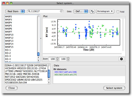
The data for 61 Vir can be accessed by searching for 61 Vir’s HD catalog number (115617):

We’ve been observing 61 Vir with both the Keck Telescope (the 77 green points) and the AAT Telescope (the 106 blue points) since 2005. The star’s location in the sky is near the celestial equator, and so it can thus be observed both from the Northern Hemisphere and from the Southern Hemisphere. For systems that harbor low-mass planets, it’s very useful to have fully independent data sets from two or more different telescopes.

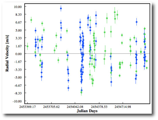
Several features of the data are evident from a simple time-series plot of the radial velocities:

First, notice the size of the error bars. Both the AAT and Keck are routinely measuring the stellar velocity to precision better than 1 meter per second. The HARPS instrument at La Silla in Chile is the only other instrument in the world that has routinely obtained radial velocity data sets that match the quality and quantity seen here. Second, notice that the velocities spanned by the data run from roughly -10 m/s to 10 m/s, which is quite a bit larger than the errors. This scatter is an initial clue up to something. Third, notice that the data is not at all evenly spaced. There have been several long observing runs at Keck, during which the star was observed every night. During late Summer and early Autumn, on the other hand, 61 Vir is behind the Sun as seen from Earth, which produces yearly gaps in the data.

The periodogram of the data exhibits a complicated structure with a number of peaks. This is an indication that we might be dealing with a multiple-planet system:

If you’ve followed through tutorials one and two on the use of the Systemic Console, you’ll likely find it straightforward to locate three planets in the data set. A simple strategy of successively fitting the highest peak in the periodogram (and after the first planet, the residuals periodogram) will quickly lead to a three planet fit that’s a match (to within the uncertainties) to the fit that’s reported in our discovery paper.

The planets in the data produce radial velocity amplitudes that are among the lowest yet reported (the current record-holder is Gliese 581e, which has K=1.9 +/- 0.2. whereas the 4.21-day planet orbiting 61 Vir has K=2.2 +/- 0.2 ). Because of these low amplitudes, it will require more observations to pin down with confidence whether the planets are on circular orbits or whether the orbits are modestly eccentric. As a result, you can get an excellent three-planet fit either by restricting system to circular orbits, or by letting the eccentricity float.

For a planetary system like 61 Vir, the signals are significantly clear-cut so that an automated routine has little difficulty in locating the best-fit configuration. One of the many new features of the console is an Automatic Fitting procedure that can be accessed under the View menu. When you select Automatic Fitting, you have the option of choosing the confidence thresholds for accepting new planets, and you have the choice of requiring that the model harbor only planets on circular orbits:

We’ve found empirically that if one requires both an F-test statistic and a False Alarm Probability below 0.1, then there’s a good chance that a system that the console finds will hold up to further scrutiny. Click OK (if you’re willing to take our word for it) and then select Run to engage the automatic fitter. The fitter adheres to a set of rules that mimic the actions of an experienced console user. It introduces planets one at a time, and cajoles the Levenberg-Marquardt optimizer to range widely over the huge space of possible system configurations. The automatic fitter rapidly converges on a three-planet system that agrees within the uncertainties with our published version:

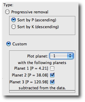
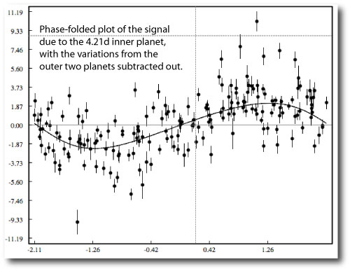
Once a trial system has been found, the console offers a huge range of options for conducting further analysis. It’s interesting, for example, to see what the individual phase-folded fits look like. This can be done by selecting Custom Plot of the Residuals under the View menu. Selecting a Custom plot as shown:

brings up a phase-folded plot of the fit of the inner 4.21-d Msin(i)=5.1 Earth Mass planet with the variations due to the outer planets subtracted out:

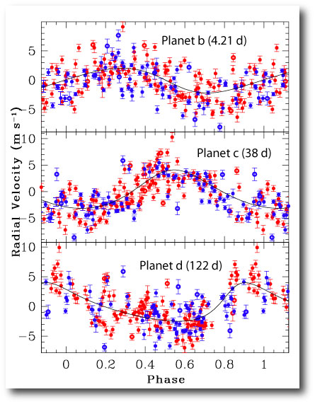
In planet detection papers, these plots have historically been presented with ~1.25 the full phase. This makes the fit stand out better to the eye. Here are the phase-folded plots from our paper which adhere to the 1.25xfull phase convention:

In our published plot, we’ve also flagged the radial velocity measurements that were noted in the observing logs as having been taken under less-than-optimal observing conditions. (These points are, however, all included in both the analysis in our paper and in the analysis performed by the console.

There’s never a free lunch. In ideal world, one would like to hold off on announcing a planetary system until a huge radial velocity data set has been accumulated. A huge data set would permit a near-perfect measurement of the planetary orbital parameters. Unfortunately, however, this isn’t possible if your planet-hunting team wants to remain competitive with the telescope Time Allocation Committees. There is a a very limited pool of nearby solar twins, and star of 61 Vir’s caliber is certainly being monitored by competing teams. One thus needs to publish forthwith once there is full confidence in a detection.

Estimation of uncertainties on the orbital parameters is of equal importance to the measurement of the orbital parameters themselves. The Systemic Console currently offers several tools for error estimation, including a bootstrap and Markov-chain Monte-Carlo estimators. Choose Bootstrap from the View menu. Click All when prompted, and then click Run.

Bootstrap Monte Carlo is a resampling method that works by successively redrawing alternative data sets from the original data set by sampling with replacement. In a redrawn data set, a given point can occur once, more than once, or not at all. A new model fit is made to each resampled data set, and the parameters of the the fits are recorded. The standard deviation of the aggregate of fitted values for a given parameter is interpreted as the 1-sigma uncertainty on the parameter. The method tends to be robust in a situations such as the one at hand where we don’t have a good a-priori estimate for the size of the uncertainty on each individual data point. Our instrumental and measurement uncertainties are well-characterized, but the uncertainty associated with astrophysical “jitter” provided by the star itself is not as well characterized. A thousand bootstrap iterations quickly generates a table of uncertainties for the orbital elements for all three planets in the system:

The console allows you to make scatter plots that illustrate the (often strong) correlations between the uncertainties on the orbital elements. For example, here’s the correlation between the bootstrapped eccentricities and the bootstrapped longitudes of periastron for the innermost planet in the system:

Even stronger correlations exist between the longitudes and the mean anomalies.

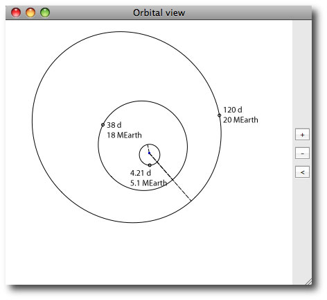
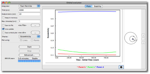
If we’ve found the planetary system that is responsible for the observed radial velocity variations, then the system should be gravitationally stable. The console has a number of tools that let the user easily perform dynamical analyses that can aid in the evaluation of stability. To get a basic flavor, choose Orbital Evolution & Stability from the View Menu. The resulting dialog box allows you to set up a numerical integration of the system and plot the results. Following the default conditions, we can watch the integration unfold, and we see that over 1,000 years, the orbital elements of the planets are varying only slowly. This is a hint (but by no means a guarantee) that the system as configured is likely to be stable…

In upcoming tutorials, we’ll delve more deeply into the console’s ability to make dynamical evaluations of planetary systems.